Named Filters are an exciting new feature which allows users to create and save specific filters directly on grid views, to then be utilized seamlessly across all policies tables, scenario items and map layers. For example, if you create a filter named “DCs” in the Facilities table to capture all entries with “DC” in their designation, this Named Filter can then be applied in a policy table, providing a dynamic alternative to the traditional Group function.

Unlike Groups, named filters automatically update: adding or removing a DC record in the Facilities table will instantly reflect in the Named Filter, streamlining the workflow and eliminating the need for manual updates. Additionally, when creating Scenario Items or defining Map Layers, users can easily select Named Filters to represent specific conditions, easily previewing the data, making the process much quicker and simpler.

In this help article, how Named Filters are created will be covered first. In the sections after, we will discuss how Named Filters can be used on input tables, in scenario items, and on map layers, while the final section contains a few notes on deleting Named Filters.

Creating Named Filters

Named Filters can be set up and saved on any Cosmic Frog table: input tables, output tables, and custom tables. These tables are found in the Data module of a Cosmic Frog model:

1. Click on the icon with 3 horizontal bars at the left top of Cosmic Frog to open the Module Menu.
2. Click on Data to open the section that contains all the tables of the Cosmic Frog model.
3. Once in the Data section, a Filter drop-down menu becomes available, the functionality of which is covered in this Help Article. When clicking on the Filter drop-down menu, users will find following filter options available to them:

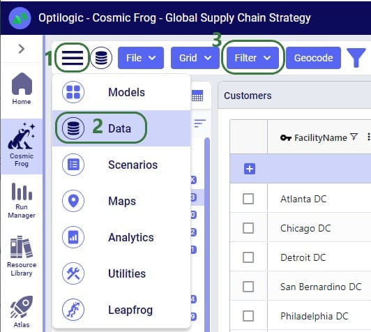
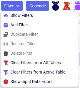
A quick description of each of the options available in the Filter drop-down menu follows here, we will cover most of these in more detail in the remainder of this Help Article:

• Show Filters: clicking on this option will show the Named Filters pane on the right-hand side of the active table. If there are any saved named filters for the table, they will be listed here. If the Named Filters pane is showing (e.g. expanded), then the option in the drop-down menu changes to Hide Filters which will collapse the Named Filters pane if user chooses this option from the drop-down menu.
• Add Filter: if a filter is applied to the active table, then choosing Add Filter will save the filter and user is prompted to give the filter a name.
• Duplicate Filter: a copy of an existing filter can be made by using the Duplicate Filter option.
• Rename Filter: use this option to change the name of an existing filter, for example if user has found the current name is no longer descriptive enough.
• Delete Filter: use this option to delete the currently selected filter. More details on deleting a Named Filter are covered in the last section of this document.
• Clear Filters from All Tables: this option will clear all filters that are currently applied to any tables, regardless of the table being open or not.
• Clear Filters from Active Table: if there are any filters applied to the active table, this option will clear those.
• Show Input Data Errors: this is a built-in filter that can be applied to input tables and will show only records which contain incorrect data. Think for example of a field containing a negative value where only positive values are valid.

Note that an additional Save Filter option becomes available in this menu in case a filter has been created (added) and next changes have been made to the table's filter conditions. The Save Filter option can then be used to update the existing named filter to reflect these changes.

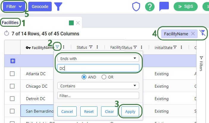
Let’s walk through setting up a filter on the Facilities table that filters out records where the Facility Name ends in “DC” and save it as a named filter called “DCs”:

1. The Facilities input table is open.
2. Click on the filter icon to the right of the Facility Name to open the filter configuration pop-up. The filter that is applied uses the "Ends with" option set to “DC”.
3. For the filter to take effect on the Facilities table, click on Apply.
4. At the right top of the Facilities table there will now be an indication that the table is filtered on the Facility Name field. Clicking on the crossed-out filter icon to the right of it will clear the filter from the table.
5. After setting up this filter, click on Add Filter in the Filter drop-down menu to save it:

1. After clicking on Add Filter in the Filter menu, the Named Filters pane on the right of the input table opens up if it was not open already. If any filters had already been saved on the Facilities table, they would be listed here. In this case, this is the first Named Filter that is being saved for the Facilities input table.
2. Type “DCs” to name the filter. After typing the name and clicking enter, it is now listed in the Named Filters pane:

1. The DCs named filter is listed in the Named Filters pane and it can be turned on (i.e. applied) or turned off (i.e. cleared) by checking and unchecking the checkbox.
2. Hovering over the name of a Named Filter will show information about the filter: it lists the field names of the fields that the filter applies to and for each field, it also lists what type of condition is applied to it. Here the field that the filter applies to is Facility Name. The type of condition can for example say “single condition” as is the case here (Ends with “DC”), or could say “or condition” in the case of multiple conditions to which or arguments are applied (e.g. facility region equals Texas or facility region equals Utah to filter out all facilities that are either in the state of Texas or in the state of Utah), etc.
3. At the right top of the table where it first indicated a filter was applied to the Facility Name field, the label now tells us that a filter named "DCs" is applied to the table. It can again be removed by clicking on the crossed-out filter icon to the right of it.

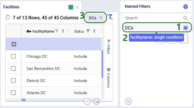
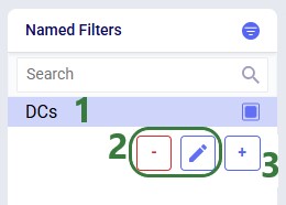
There are 3 buttons below the list of filters as follows (these were obscured by the hover text in the previous screenshot):

1. You can select a filter from the list by clicking on it. The background color will then become purple-grey instead of white.
2. When a filter is selected, the left 2 of the 3 buttons become active. These can be used to remove the filter or to rename it.
3. The third button can be used to add (save) the filter that is currently applied to the table, i.e. it is an alternative to the "Add Filter" option from the Filter menu.

There is a right-click context menu available for filters listed in the Named Filters pane, which allows the user to perform some of the same actions as those in the main Filter menu shown above:

1. These 4 options work on the currently selected filter in the list itself and can be used to duplicate, rename, save or delete the Named Filter that was right clicked on. Saving can be used if changes have been made to the filter conditions after the filter was first created to reflect those changes in the filter. An example will be stepped through further below. Deleting a Named Filter will be covered in the last section of this document.
2. Clicking on the Hide Filters option will collapse the Named Filters pane.
3. If a filter is applied to the input table, clicking on Add Filter will add a Named Filter for it to this list.
4. The Clear Filters from All Tables and Clear Filters from Active Table options are available here too, which will achieve the same as the corresponding options in the main Filter menu, explained further above.

Named Filters can use filtering conditions that are applied to multiple fields in a table. The next example shows a Named Filter called “CZ2* Space Suit demand >6k” on the Customer Demand input table which uses filtering conditions on three fields:

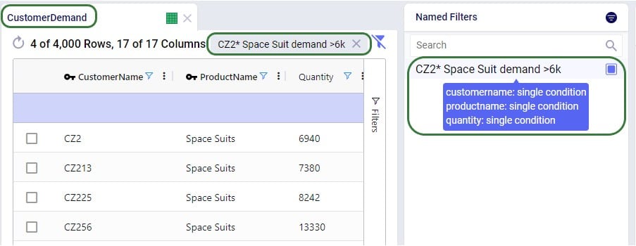
Conditions were applied to 3 fields in the Customer Demand table, as follows: 1) Customer Name Begins With “CZ2”, 2) Product Name Contains “Space”, and 3) Quantity Greater Than “6000”. The resulting filter was saved as a Named Filter with the name “CZ2* Space Suit demand >6k” which is applied in the screenshot above. When hovering over this Named Filter, we indeed see the 3 fields and that they each have a single condition on them.

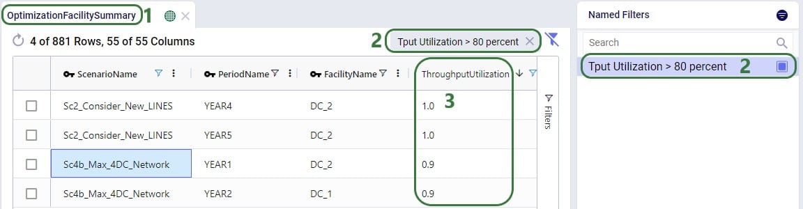
Besides being able to create Named Filters on input tables, they can also be created on output and custom tables. On output tables this can for example expedite the review of results after running additional scenarios where one can apply a pre-saved set of Named Filters one after the other once the runs are done instead of having to re-type each filter that shows the outputs of interest each time. This example shows a Named Filter on the Optimization Facility Summary output table to show records where the Throughput Utilization is greater than 0.8:

1. We are on the Optimization Facility Summary output table.
2. A Named Filter with the name “Tput Utilization > 80 percent” is applied.
3. In this example this results in 4 records where the utilization was more than 80%.

‍

Applying Multiple Named Filters

Next, we will see how multiple Named Filters can be applied to a table. In the example we will use, there are 4 Named Filters set up on the Facilities table:

1. There are 4 Named Filters set up on the Facilities table: one named DCs that filters out all records where the Facility Name ends with DC, one named Ports that filters out all records where the Facility Name ends with Port, one named Factories that filters out all records where the Facility Name ends with Factory, and one named USA locations that filters out all records where the Country is USA. This last one, "USA locations", has been applied to the table.
2. At the top right of the table, we also see that the "USA locations" Named Filter is applied to the table.
3. We see that all 9 filtered records have Country = USA.
4. We also notice that these locations are of different types: 7 DCs, 1 Factory, and 1 Port.

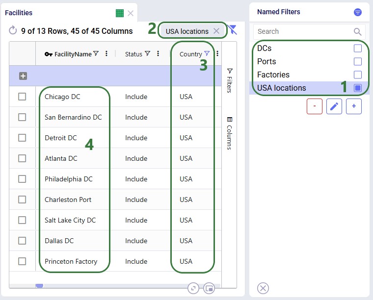
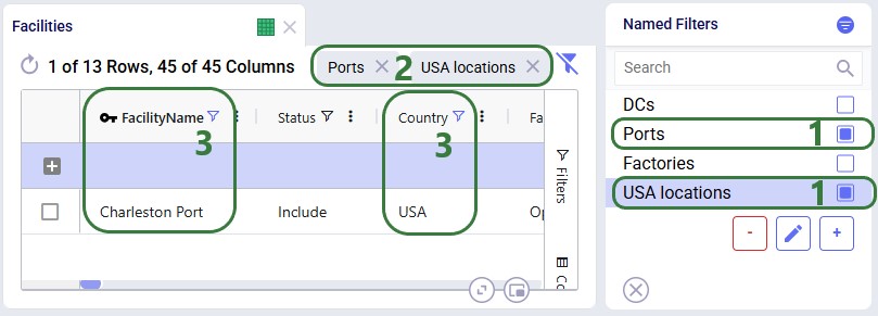
Next, we will apply another Named Filter in addition to this first one ("USA locations"). How the Named Filters work together depends on if they are filtering on the same field or on different fields:

• When multiple Named Filters are applied and they are using different fields to filter the table on, they act as AND statements: only records that match the criteria of all Named Filters are shown.
• When multiple Named Filters are applied and they are using the same field to filter the table on, they act as OR statements: records that match any of the applied Named Filters are shown.

Now, if we want to filter out only Ports located in the USA, we can apply 2 of the Named Filters simultaneously:

1. The checkboxes of both the "Ports" and "USA locations" Named Filters are checked and therefore both are applied to the table.
2. At the top right of the table, we again see that these 2 Named Filters are applied, and if desired we can clear them here by clicking on the crossed-out filter icon.
3. The filter icons to the right of the field names for the Facility Name and Country fields are blue, indicating a filter is applied to both. And we can see that indeed only Ports in the USA are filtered out (there is only 1 record that matches the filter criteria in this model). In this case the 2 Named Filters filter on different fields and therefore act as an AND statement: only records for which the facility name ends with "Port" AND for which the Country is "USA" are shown.

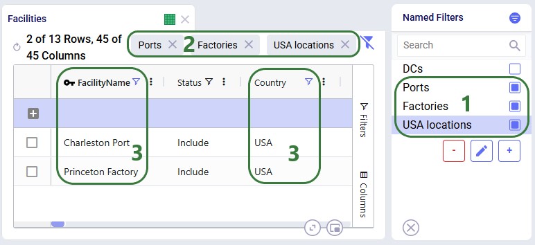
To show an example of how multiple named filters that filter on the same field work, we will add a third Named Filter:

1. In addition to the 2 Named Filters which were already applied in the previous screenshot, "USA locations" and "Ports", now we have applied a third too, the one named "Factories".
2. The three filters are listed at the right top again.
3. Now we see that ports in the USA as well as factories in the USA are being shown. The "Ports" and "Factories" Named Filters filter on the same field (Facility Name) which acts as an OR statement: show records where (facility name ends with "Port" OR "Factory") AND Country equals "USA".

Editing a Named Filter

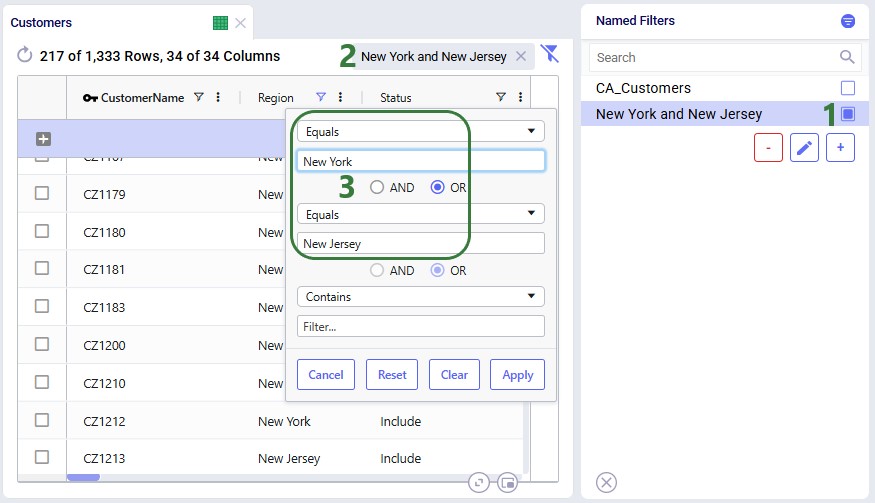
To alter an existing filter, we can change the criteria of this existing filter, and then save the resulting filter, replacing the original Named Filter. Let’s illustrate this through an example: in a model with about 1.3k customers in the US, we have created a Named Filter “New York and New Jersey”, but later on realize that this filter also includes customers in New Hampshire and New Mexico:

1. A filter is applied to the Region field (which are states in the US) to filter out all records where the Region value contains the text "New".
2. The filter has been added as a named filter, which is called "New York and New Jersey".

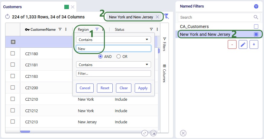
In reality, this filter also filters out customers located in the regions (states) of New Hampshire and New Mexico in addition to those in New York and New Jersey. So, the next step is to update the filter to only filter out the New York and New Jersey customers:

1. The filter on the Region field is changed so that only records where the Region value equals "New York" or where it equals "New Jersey" are filtered out.
2. When changing the filter criteria, automatically, the "New York and New Jersey" named filter's checkbox is unchecked, since the table is not filtered for its original filter condition anymore.
3. The named filter is also not shown as the label at the right top of the table anymore and the label has reverted to indicating which field the table is filtered on.

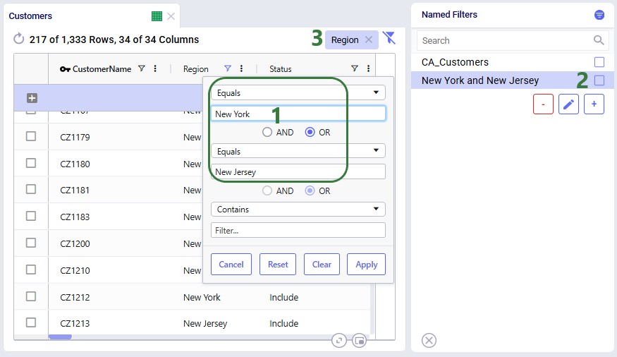
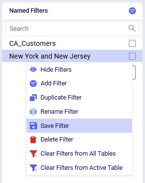
Next, we can use the Save Filter option from either the Filter menu drop-down list or the context menu after right-clicking on the filter in the Named Filters pane to update the existing "New York and New Jersey" named filter to use the updated condition. The following screenshot shows the latter method:

After choosing Save Filter from the context menu, the following message is shown for the user to confirm they want to overwrite the original named filter using the current filter conditions:

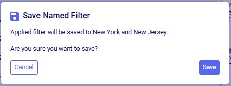
After clicking Save, the existing named filter has been updated:

1. Automatically, the checkbox of the filter has been checked again.
2. The label at the right top of the table also reflects the name of the applied named filter again.
3. Checking the filter on the Region field we see that it is the updated one which only filters out records where the customer is located either in New York or in New Jersey.

So far, the only examples were of filters applied to one field in an input table. The next example shows a Named Filter called “CZ2* Space Suit demand >6k” on the Customer Demand input table which uses filtering conditions on multiple fields:

Conditions were applied to 3 fields in the Customer Demand table, as follows: 1) Customer Name Begins With “CZ2”, 2) Product Name Contains “Space”, and 3) Quantity Greater Than “6000”. The resulting filter was saved as a Named Filter with the name “CZ2* Space Suit demand >6k” which is applied in the screenshot above. When hovering over this Named Filter, we indeed see the 3 fields and that they each have a single condition on them.

Besides being able to create Named Filters on input tables, they can also be created on output and custom tables. On output tables this can for example expedite the review of results after running additional scenarios where one can apply a pre-saved set of Named Filters one after the other once the runs are done instead of having to re-type each filter that shows the outputs of interest each time. This example shows a Named Filter on the Optimization Facility Summary output table to show records where the Throughput Utilization is greater than 0.8:

1. We are on the Optimization Facility Summary output table.
2. A Named Filter with the name “Tput Utilization > 80 percent” is applied.
3. In this example this results in 4 records where the utilization was more than 80%.

Input Data Errors Filter

The last option of Show Input Data Errors in the Filter menu creates a special filter named ERRORS and filters out records in the input table it is used on that have errors in the input data. This can be very helpful as records with input errors may have these in different fields and the types of errors may be different, so a user is not able to create 1 single filter that would capture multiple different types of errors. When this filter is applied, any record that has 1 or multiple fields with a red outline will be filtered out and shown. Hovering over the field gives a short description of the problem with the value in the field.

1. The Show Input Data Errors option from the Filter menu was used while on the Products table. This special filter is called “ERRORS” and has its own red icon so it is easily recognized.
2. In this case one record is shown. The Unit Price field of this record has a red outline indicating its value is troublesome. Hovering over the field it says “cannot be negative”. Updating the Unit Price to a value => 0 will resolve the input data error.

‍

Using Named Filters on Input Tables

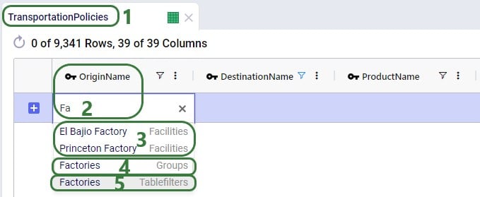
Named Filters for certain model elements (i.e. Customers, Facilities, Suppliers, Products, Periods, Modes, Shipments, Transportation Assets, Processes, Bills Of Materials, Work Centers, and Work Resources) can be used in other input tables, very similar to how Groups work in Cosmic Frog: instead of setting up multiple records for individual elements, for example a transportation policy from A to B for each finished good, a Named Filter that filters out all finished goods on the Products table can be used to set up 1 transportation policy for these finished goods from A to B (which at run-time will be expanded into a policy for each finished good). The advantage of using Named Filters instead of Groups is that Named Filters are dynamic. If records are added to tables containing model elements and they match the conditions of any Named Filters, they are automatically added to those Named Filters. Think for example of Products with the pre-fix FG_ to indicate they are finished goods and a Named Filter “Finished Goods” that filters the Product Name on Begins With “FG_”. If a new product is added where the Product Name starts with FG_, it is automatically added to the Finished Goods Named Filter and anywhere this filter is used this new finished good is now included too. We will look at 2 examples in the next few screenshots.

1. We are on the Transportation Policies input table.
2. When typing 2 characters or more into a field, here the Origin Name field, a drop-down of matches from different tables, groups, and named table filters is populated. Here “Fa” has been typed in.
3. There are 2 matches from the Facilities table: 2 records have a Facility Name that contains “Fa”, El Bajio Factory and Princeton Factory. Either of these can be chosen from the list to set up a transportation policy for that individual factory.
4. There is 1 match from the Groups table: 1 record has a Group Name that contains “Fa” and is of a Group Type that can be used as the origin for a transportation policy (Group Types of Facilities, Suppliers and Sources can be used): the group named Factories which contains the El Bajio and Princeton factories. If this group is chosen, a transportation policy is set up for these 2 factories. If a new factory is added to the Facilities table, it will not automatically be added to the Factories group and therefore this transportation policy will not be updated to include the third factory.
5. There is 1 match from the Tablefilters (= Named Filters) present in the model in tables that are suitable to function as origins in a transportation policy (the Facilities and Suppliers tables). The Named Filter is called Factories and this is a filter with a condition on the Facility Name field on the Facilities table for Ends With “Factory”. If this Named Filter is chosen, a transportation policy is set up for these 2 factories. If a new factory is added to the Facilities table and the name ends with “Factory”, it will automatically be added to this Factories Named Filter and therefore this transportation policy will also be automatically updated to include the third factory.

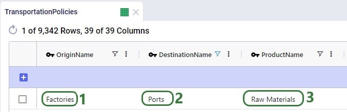
The completed transportation policy record uses Named Filters for the Origin Name, Destination Name, and Product Name, making this record flexible as long as the naming conventions of the factories, ports, and raw materials keep following the same rules.

1. The Factories Named Filter from the Facilities table where the condition of Ends With “Factory” is applied to the Facility Name field.
2. The Ports Named Filter from the Facilities table where the condition of Ends With “Port” is applied to the Facility Name field.
3. The Raw Materials Named Filter from the Products table where the condition of Begins With “RM” is applied to the Product Name field.

The next example is on one of the Constraints tables, Production Constraints. On the Constraints tables, the Group Behavior fields dictate how an element name that is a Group or a Named Filter should be used. When set to Enumerate, the constraint is applied to each individual member of the group or named filter. If it is set to Aggregate, the constraint applies to all members of the group or named filter together. This Production Constraint states that at each factory a maximum amount of 150,000 units over all finished goods together can be produced:

1. We are on the Production Constraints input table.
2. The Facility Name is set to the Factories Named Filter from the Facilities table (condition on Facility Name for Ends With “Factory”). Since its Group Behavior field is set to Enumerate, the constraint applies to each factory of the Named Filter individually.
3. The Product Name is set to the Finished Goods Named Filter on the Products table (condition on Product Name for Does not contain “RM”). Since its Group Behavior field is set to Aggregate, the constraint applies to the 3 finished goods in the model together.
4. The Constraint Type and Constraint Value fields set the upper limit of 150,000 units.

Using Named Filters in Scenario Items

When setting up a scenario item, previously, the records that the scenario item’s change needed to be applied to could be set by using the Condition Builder. Now users have the added option to use a saved Named Filter instead, which makes it easier as the user does not need to know the syntax for building a condition, and it also makes it more flexible as Named Filters are dynamic as was discussed in the previous section. In addition, users can preview the records that the change will be made to so the chance of mistakes is reduced.

Please note that a maximum of 1 Named Filter can be used on a scenario item.

The following example changes the Suppliers table of a model which has around 70 suppliers, about half of these are in Europe and the other half in China:

1. We are creating a Scenario Item named “Exclude China Suppliers” (Module Menu > Scenarios, Scenario Menu > New Item).
2. We select Suppliers as the Table Name as this is the table we want to make the changes to.
3. We type status = ‘Exclude’ in the Actions box since we want to change the Status of a subset of Suppliers (those located in China) from Include (which is the Status in the Suppliers table) to Exclude.
4. In the Conditions section we choose to use Named Filters to set the condition(s) of which records on the Suppliers table should have their Status set to Exclude.
5. Click on the down caret to open the Named Filters drop-down list.
6. There are 2 Named Filters listed here from the Suppliers table. The Europe Suppliers Named Filter has a condition on the Country field of Does not contain “China” and the China Suppliers Named Filter has a condition on the Country field of Equals “China”. We choose the China Suppliers Named Filter by checking its checkbox:

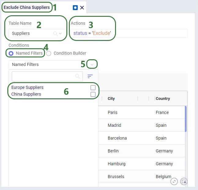
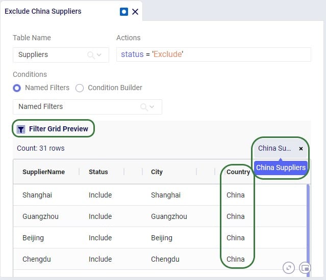
The Named Filters drop-down collapses after choosing the China Suppliers Named Filter as the condition, and now we see the Preview of the filtered grid. This is the Suppliers table with the Named Filter China Suppliers applied. At the right top of the grid the name of the applied Named Filter(s) is shown, and we can see that in the preview we indeed only see Suppliers for which the Country is China. So these are the records the change (setting Status = Exclude) will be made to in scenarios that use this scenario item.

A few notes on the Filter Grid Preview:

• The column(s) to which condition(s) are applied are indicated with the filter icon next to the field name(s).
• Users can resize the columns by clicking on the horizontal bars in between them and then dragging those left or right.
• Users can sort them by clicking on the field names, clicking once sorts in ascending order, clicking again in descending order, and clicking one more time takes the sort off. Sorting by multiple columns is possible too: after sorting the first column, hold down the Ctrl and Shift keys and then click on the second column to sort by, etc.
• Users cannot change the order of the columns in the grid.

Using Named Filters on Map Layers

Besides using Named Filters on other input tables and for setting up conditions for scenario items, they can also be used as conditions for Map Layers, which will be covered in this final section of this Help Article. Like for scenario items, there is also a Filter Grid Preview for Map Layers to double-check which records will be filtered out when applying the condition(s) of 1 or multiple Named Filters.

In this first example, a Named Filter on the Facilities table filters out only the Facilities that are located in the USA:

1. We are on the Map named Supply Chain (Module Menu > Maps, click on the Map named Supply Chain), and are adding a new Layer named “USA Facilities” to it (Map Menu > New Layer).
2. In the Layer configuration pane on the right, we are on the Condition Builder (left icon of the 3 icons at the top right).
3. For Layer Name, “USA Facilities” was typed in.
4. Facilities is selected as the Table Name from which the later will be generated.
5. Besides the Condition Builder which was already available to users to manually type in any conditions to be applied to the Facilities table when adding the Map Layer, users now have the option to use Named Filters instead, which is the option selected in this example.
6. The “USA locations” Named Filter was selected from the Named Filters drop-down list. This is a Named Filter on the Facilities table with a condition on the Country field of Equals “USA”.
7. Here the Show Grid Preview option is turned on, which changes the view of the map to the Filter Grid Preview (by default it is off and the changes will be immediately visible on the map).
8. Since Show Grid Preview was turned on, we see the Filter Grid Preview here.
9. At the top right of the filtered preview of the Facilities table, it is indicated that a filter called “USA locations” is applied.
10. In the Grid Preview itself we see that 9 locations match the filter’s condition of Country = USA, and therefore these 9 locations will be shown on this Map Layer. Switching the Show Grid Preview off, the map appears:

1. We are still on the Supply Chain map.
2. The USA Facilities layer was added and is the only one that is enabled for the Supply Chain map currently.
3. As mentioned, the Show Grid Preview has been turned off again.
4. The map shows the 9 locations that are based in the USA.

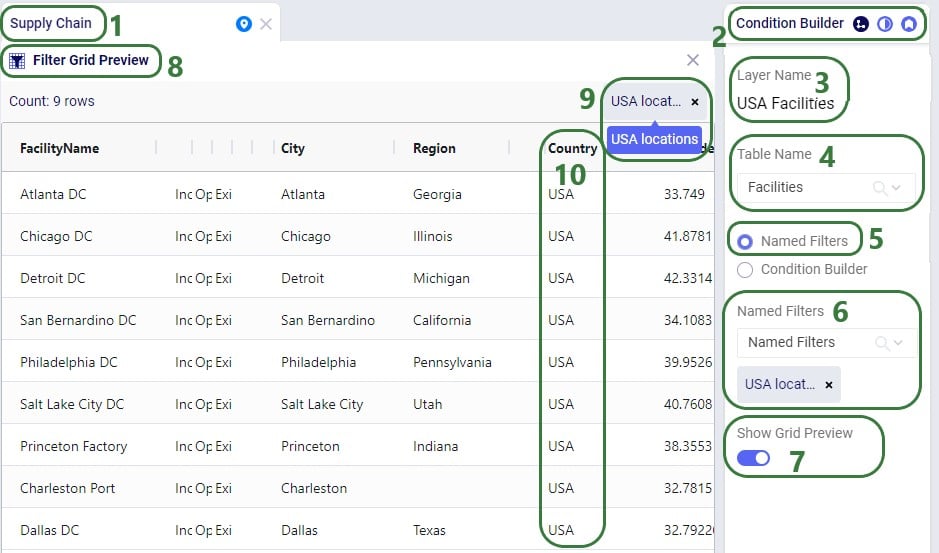
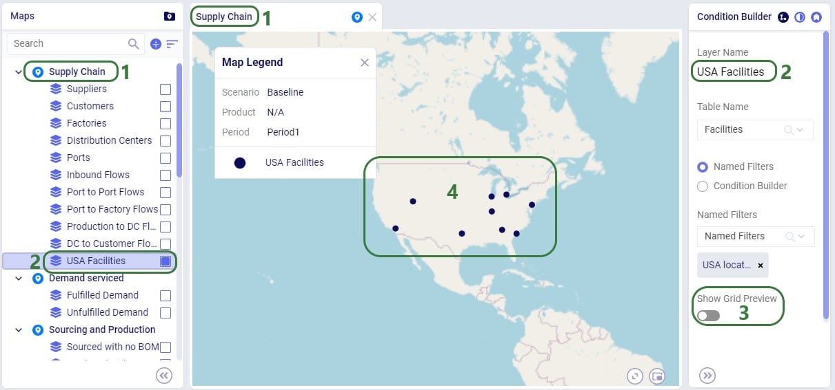
Another example of the same model is to use a different Named Filter from the Facilities table to show only Factories on the map:

1. We are on the Supply Chain map still.
2. A Layer named Factories is the only one that is enabled.
3. Named Filters are used again as the condition.
4. The Factories Named Filter on the Facilities table is used to only show the 2 factories in the model (in El Bajio and Princeton). The condition applied to the Facility Name field is Ends With “Factory”.

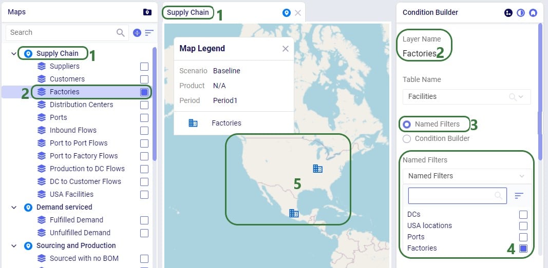
Applying multiple Named Filters on maps works the same way as for tables:

• When multiple Named Filters are applied and they are using different fields to filter the underlying table on, they act as AND statements: only records that match the criteria of all Named Filters are shown.
• When multiple Named Filters are applied and they are using the same field to filter the underlying table on, they act as OR statements: records that match any of the applied Named Filters are shown.

For example, applying the Ports and Factories filters will show all Ports (4 in total, 2 not shown in the screenshot as they are in Europe and China) and all Factories (2) - these are 2 filters on the same field (facility name) and are therefore OR-ed:

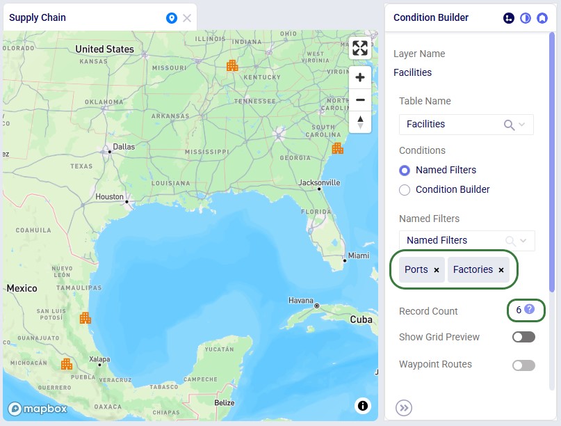
Now, when we also enable the US Locations filter in addition, only the Port and Factory in the US are shown on the map - the US Locations filter applies to a different field (country) and is therefore AND-ed with the other 2:

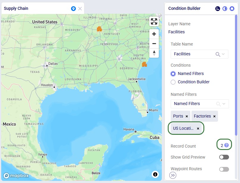
The same notes that were listed for the Filter Grid Preview for scenario items apply to the Filter Grid Preview for Map Layers too: columns with conditions have the filter icon on them, users can resize and (multi-)sort the columns, however, re-ordering the columns is not possible.

Deleting a Named Filter

Named Filters can be deleted, and this affects other input tables, scenario items, and map layers that used the now deleted Named Filter(s). This will be explained further in this final section of the Help Article on Named Filters.

A Named Filter can be deleted by using one of three methods:

1. Use the main Filter menu’s “Delete Filter” option
2. Choose the "Delete Filter" option from the right-click context menu of a Named Filter in the Named Filters pane.
3. Select the named filter in the Named Filters pane and then click on the "Delete Filter" button with (the one with the minus sign on it; the first of the 3 buttons underneath the list of named filters).

After choosing to delete a named filter, the following message comes up to ask the user for confirmation. In this example we are deleting the filter named "New York and New Jersey" which is a filter on the Customers input table:

‍

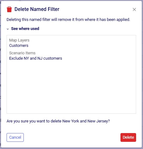
The message will let the user know if the named filter that is about to be deleted was used in any Map Layers and/or Scenario Items. If so, it lists the names of these layers/items in the "See where used" section which can be expanded and collapsed by clicking on the caret symbol. Note that currently this message does not indicate if the named filter is used in any input tables.

The results of deleting a Named Filter that was used are as follows:

1. Deleting a Named Filter that was used on another input table: the record(s) that use the Named Filter are left unaltered in the other input tables. As these are now invalid, they will be ignored during a model run.
2. Deleting a Named Filter that was used as a condition in a scenario item: the Named Filter is not applied anymore, so its condition is no longer placed on the scenario item and the change of the scenario item will be applied to the whole table now.
3. Deleting a Named Filter that was used as a condition for a map layer: the named filter is no longer applied to the map layer(s) it was used on. For example if the "New York and New Jersey" named filter of the Customers table was applied to a map layer showing customer locations, it will now show all customers instead of just the ones in New York and New Jersey.

Overview

The Modeler Agent is one of Ada’s AI-powered supply chain modeling specialists. It helps users build, validate, troubleshoot, run, analyze, and automate Cosmic Frog network optimization (Neo) and transportation optimization (Hopper) models. The Modeler Agent accelerates the entire modeling lifecycle – from raw operational data to optimization-ready model construction and scenario analysis – while improving model quality, traceability, and reproducibility. By combining supply chain domain knowledge with direct platform capabilities, it helps teams move from messy source data to solver-ready models faster and with fewer manual hand-offs.

The agent can be accessed by chatting with Ada in the next generation Optilogic platform and via Run AI Agent tasks in DataStar.

Why It’s Useful

Users get leverage in these main areas:

1. Faster model construction: The agent helps users build Cosmic Frog models (ANURA schema) more quickly by guiding schema mapping, validation, and preprocessing readiness.

2. Schema-first correctness: The agent will push to verify the actual  table/column requirements instead of guessing.

3. Faster debugging: When outputs are empty or a run fails, the agent focuses on the most common root causes: preprocessing/validation drops, missing connectivity, wrong enumerations/UOM, period mistakes, or broken relationships.

4. Repeatable pipelines: If you want automation, the Agent can help create a Datastar macro so your model build is reproducible (build → validate → export → run).

5. Better visibility and traceability: The platform logs agent plans, tool usage, actions, and outputs so modeling work can be reviewed and audited.

Key Capabilities

Data → Model mapping

• Map raw/staging tables to ANURA inputs (customers, facilities, products, demand, shipments, policies, etc.)
• Identify missing structure and propose the least-assumptive proxy inputs (with clear labeling)

Validation & feasibility checks

• Check required fields, enumerations, master-table relationships, UOM consistency, and period/horizon alignment
• Pre-solve viability checks (e.g., demand has a feasible path to supply)

Scenario & policy authoring (conceptual + implementation guidance)

• Help design and create scenarios (what changes, where, and expected affected-row counts)
• Help interpret how policies/constraints change the feasible network

Engine execution support

• Guide Neo/Hopper run readiness and interpret outputs (and treat “empty outputs” as a failure signal to diagnose)

Workflow automation (DataStar)

• Create repeatable model-build workflows (Macros & Tasks) in DataStar
• Emphasize “transform in staging, export final tables to ANURA”

Reporting and documentation

• Generate markdown summaries of assumptions and findings
• Document trade-offs and validation outcomes

Using the Modeler Agent

There are two ways to access the Modeler Agent:

1. Through chatting with Ada in the next generation Optilogic platform
2. By using Run AI Agent tasks within DataStar

Both ways will be explained: via chat first, then the DataStar workflow, followed by an overview of the main differences between the 2 methods.

Using the Modeler Agent within the Chat UI

It is recommended to be somewhat familiar with Ada and how to talk to her in the chat UI before diving into this content. Please see the Getting Started with Ada & Agentic AI article, and in particular its How to Use Ada section.

Once logged into the next generation Optilogic platform at https://ai.optilogic.app, you can start chatting with Ada leveraging the Modeler Agent right away from the central part of the Home page.

Here, our example is of a new modeler who inherited a work in progress model to evaluate and optimize their company's manufacturing footprint. They have the Cosmic Frog model which is partially built and a DataStar project with both raw historical and master data, and a set of previously cleaned tables.

1. If unsure how to start, or if you are just exploring, you can use 1 of the example prompts to get going.
2. Underneath the prompt textbox, we can:
   
   1. Select the interaction Style to use. These behave differently in how verbose the agent’s answers will be and how often user confirmation/feedback will be sought before proceeding. See the Create your First Prompt section in the Getting Started with Ada article for more details. Typically, Scout (the default style) works well for users experienced with Optilogic tools who are starting to use AI.
   2. Connect to 1 or multiple Cosmic Frog models, DataStar projects, or Postgres databases. The prompt can refer to these and data can be moved from one database to another. In this example, we have connected to 2 databases: 1 Cosmic Frog model and 1 DataStar project; see next screenshot.
   3. Choose the agent to use for the prompt; we are using the Modeler Agent here.
3. Type your question/task into the prompt textbox.
4. Click on the submit button.

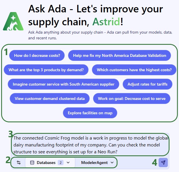
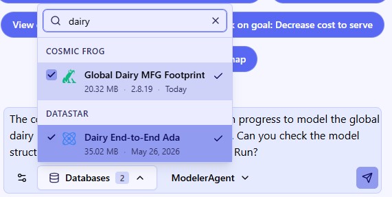
Our 2 connected databases are shown in this screenshot:

After submitting a prompt, the Modeler Agent will start processing and formulating a response; the following 3 screenshots show the full response:

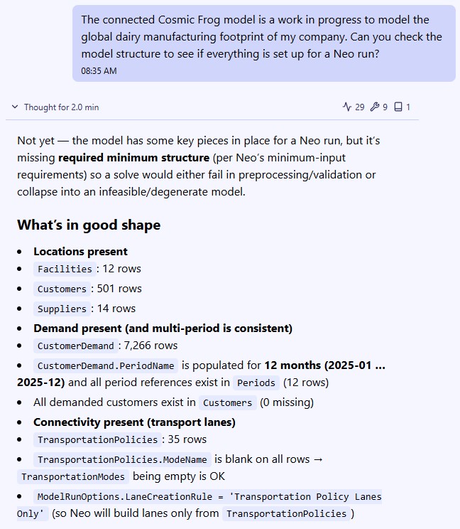
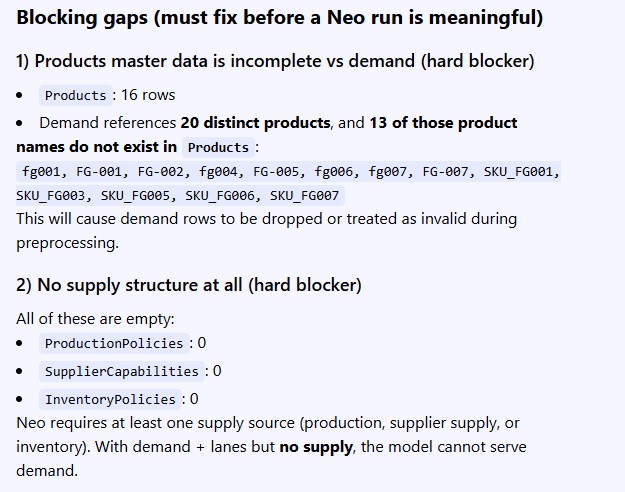
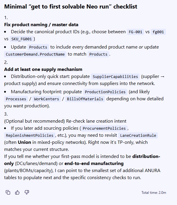
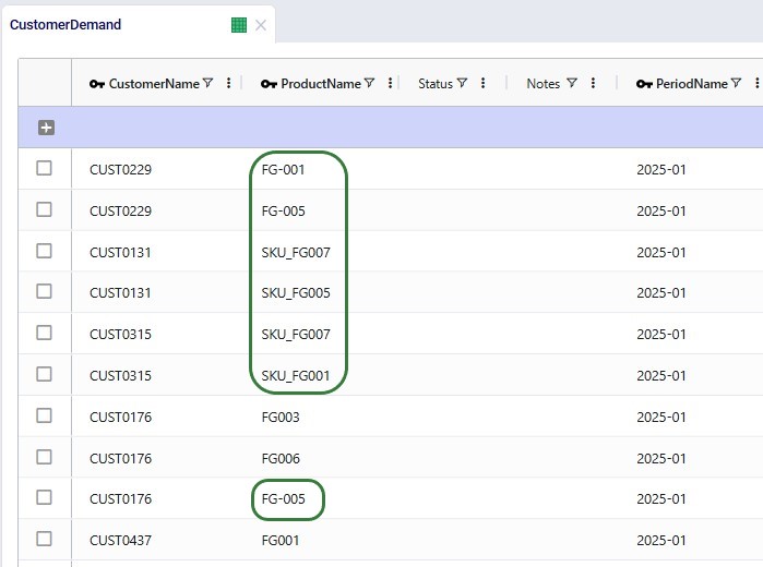
We now understand there are several issues that need to be addressed before we can attempt a first model run. First, the user decides to focus on the product name problem identified in the Customer Demand table. To understand the problem, we first have a look at the Customer Demand table in the Cosmic Frog model and notice that whereas all finished goods should follow the naming convention of FGXXX, many do not:

Since we are not familiar with the data in the DataStar project, we ask the Modeler Agent if there are tables that can help resolve the product naming problem:

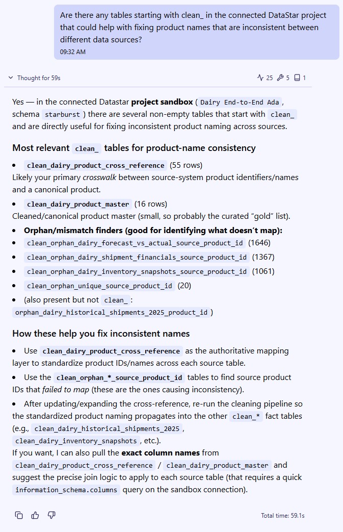
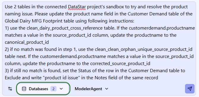
We then have a look at the mentioned tables in the DataStar project and identify the 2 we think can be used as lookups to fix the incorrect product names:

The response does not yet make any changes, but summarizes what they will be and asks us to confirm before making the changes:

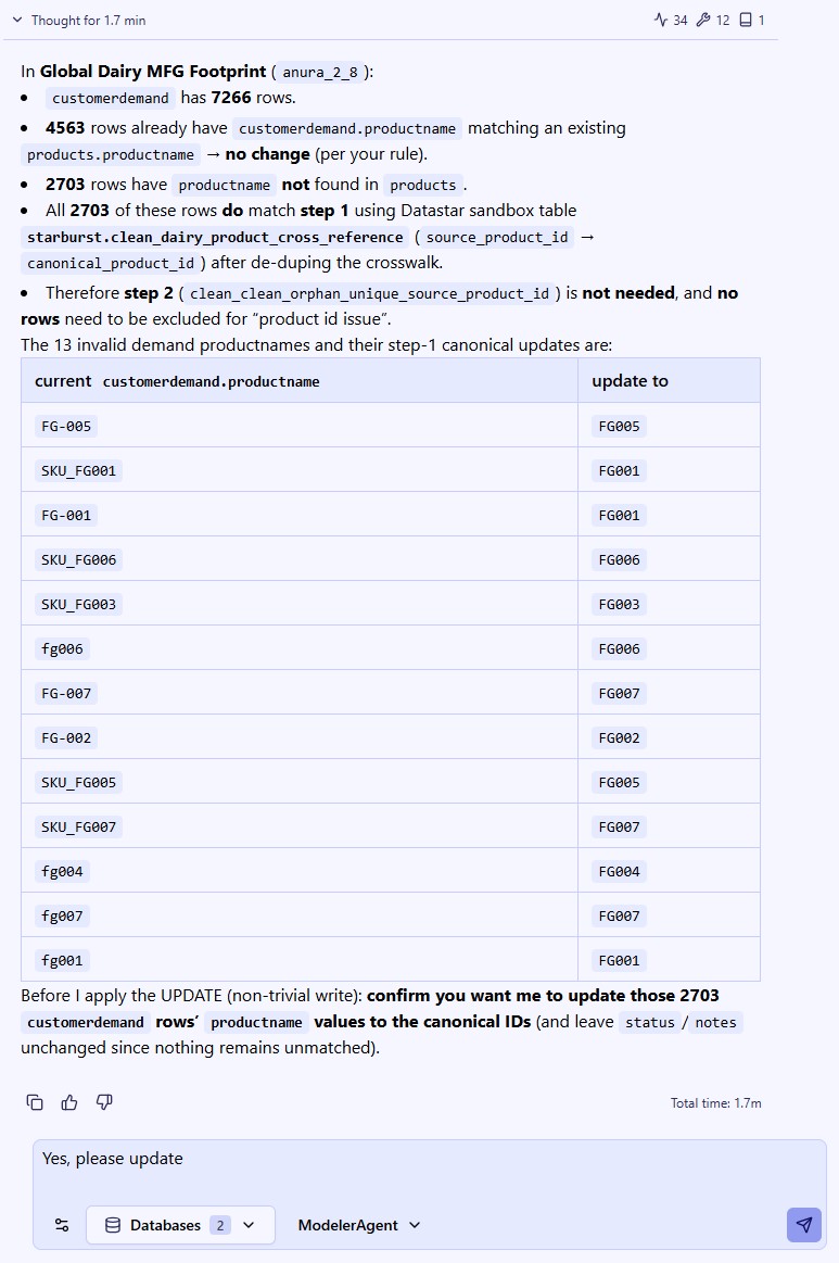
After submitting the confirmation, the changes are made:

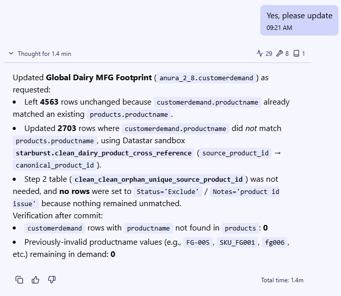
And checking the Customer Demand table in Cosmic Frog, we see the product naming is now consistent. The names outlined in green were incorrect previously (see screenshot above):

Using the Modeler Agent within DataStar

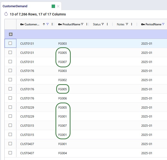
Accessing the Modeler Agent through DataStar is done via a Run AI Agent task:

1. From the Tasks tab, click on a Run AI Agent task and drag it onto the Macro canvas to add it to your active Macro.
2. Start configuring the task on the Configuration tab that is now active:
   
   1. Type the task’s name in the Name textbox.
   2. In the Select Utility section, choose Modeler Agent from the list of available agents by clicking on it.

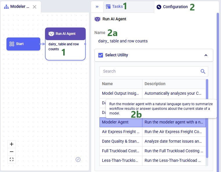
Next, configure the other parts of the task:

1. Expand the Configure Utility part if not yet expanded.
2. From the drop-down list, select the database you want the modeler agent to use. This can be a Cosmic Frog model, a DataStar project, or a Postgres database.
3. Type your question/task in the Query field.
4. Choose how verbose the agent’s output should be, concise or detailed.
5. In the Run Configuration section, users can add Tags to facilitate finding job runs, set a Timeout for the task, and set the Resource Size to use. Note that for most Run AI Agent tasks, the Resource Size will need to be set to XS or higher.
6. Optionally, add notes about this task in the Notes part.

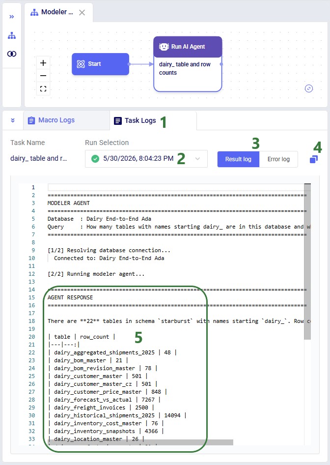
After running a Run AI Agent task, the Task Logs tab located underneath the Macro canvas will show the log that contains the Modeler Agent’s response:

1. Click on the Task Logs tab.
2. The log of the most recent run of the task will be shown, use the Run Selection drop-down to see results of prior runs.
3. The Result Log will be shown by default. When troubleshooting any issues, clicking on the Error log to review it can be helpful.
4. To copy the task log, use this copy button.
5. The asked for output (row counts of tables starting with dairy_) are listed in the Agent Response part of the log.

‍

‍

Modeler Agent Usage: Chat UI vs DataStar

There are a few differences to keep in mind when running the Modeler Agent either via the chat with Ada UI or from within DataStar:

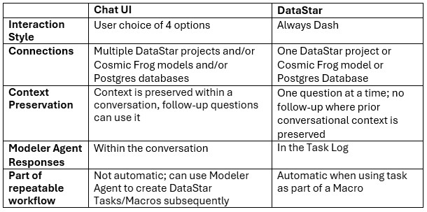
Recommendation: Use the chat UI to develop and refine a prompt, then transfer the working prompt into a DataStar Run AI Agent task once you want the workflow to become repeatable.

Best Practices for Prompt Writing

The general Best Practices, Tips & Tricks, and Current Limitations and Known Behaviors included in the Getting Started with Ada documentation also apply to the Modeler Agent. In addition, we recommend providing the Modeler Agent with structured context. The more structured context provided, the faster and more accurately it can help.

Specify the engine and objective

Better:
“Using Neo, minimize total landed cost while meeting all customer demand.”

Worse:
“Optimize my supply chain.”

Specify grain and keys

Better:
“Demand is customer-product-month keyed by (customer_id, sku, month).”

Worse:
“Here’s demand data.”

Clarify constraints and assumptions

Examples:

• Can demand go unmet?
• Is single-sourcing required?
• Can products co-load on vehicles?
• Are facilities fixed or selectable?

Separate staging from ANURA model tables

Transform and cleanse data in staging layers whenever possible and export finalized structures into ANURA.

Ask for evidence

Request:

• Row counts
• Distinct keys
• Validation summaries
• Failing rows

rather than only asking:
“Is it valid?”

Prefer incremental changes

Better:
“Fix these 3 fields.”

Worse:
“Rebuild the whole model.”

Top 10 Starter Prompts

Inspect an existing model

“Inspect my model {database name}: what ANURA tables are populated, and what are row counts by table?”

Identify minimum required inputs

“I want to run {Neo|Hopper} for {problem statement}. What are the minimum ANURA input tables and critical required fields?”

Map raw source data into ANURA

“Here are my source tables {table list} with keys {keys}. Propose a mapping into ANURA tables for {engine} and list assumptions and gaps.”

Validate referential integrity

“Check that all {demand table} references exist in {Customers, Products} and show missing keys.”

Diagnose empty outputs

“My run completed but outputs are (partially) empty. Walk me through the most likely causes and the checks to confirm each.”

Troubleshoot Infeasibility (Neo) / Unrouted Shipments (Hopper)

“My model is infeasible. Help me troubleshoot.”

“About 60% of shipments in scenarios 2 and 3 are unrouted. Diagnose why.”

Create scenarios

“Create a set of scenarios where the 5 currently excluded DCs are set to Consider and demand is increased by 10%, 30%, and 50%.”

Configure Hopper inputs

“I have shipments at the weekly level and 5 different types of assets. What ANURA tables do I need for Hopper?”

Build a DataStar workflow

“Design a DataStar macro that builds Cosmic Frog model-ready Facilities and Products tables from the clean_DC_Master, clean_MFG_Master and clean_SKU_Master tables in this DataStar project’s sandbox and exports them into the EMEA Neo Cosmic Frog model.”

Output analysis and reporting

“Analyze the outputs of the Neo scenarios in the Global Supply Chain Strategy model. Generate a report for the leadership team which compares the scenarios and focuses on the biggest shifts and main KPIs.”

‍

Common Pitfalls Avoided

Modeling Mistakes

The Modeler Agent helps supply chain modeleres avoid common modeling mistakes such as:

• Guessing ANURA schema instead of reading metadata
• Populating fields that preprocessing derives automatically based on defaults
• Treating sentinel values like ALL as real master-data values
• Performing transformations directly inside ANURA model tables
• Launching solves before confirming connectivity (e.g. demand has a valid supply path)
• Mixing incompatible units of measure
• Misaligning periods or horizons in multi-period models

Running a Model Too Soon

Many optimization issues originate during preprocessing rather than inside the solver itself. Preprocessing typically:

• Applies defaults
• Validates relationships
• Resolves references
• Validates enumerations
• Filters invalid records
• Builds optimization-ready structures

Common preprocessing-related symptoms include:

• Empty outputs
• Missing flows
• Dropped rows
• Missing periods
• Zero-row intermediate structures

The Modeler Agent is designed to diagnose these issues before expensive solves are executed whenever possible.

Example Typical Model Build Workflow

1. State the decision question
   
   • Example: “We need to build a Cosmic Frog model to answer the question of which DC should serve which customer(s) to minimize cost subject to capacity.”
2. Name the engine
   
   • Neo for network optimization; Hopper for transportation optimization

3. Describe your data and where it lives
   
   • What tables exist, what connection/schema, what grain (SKU vs product family?, day / week / month?)

4. Ask for a check before running
   
   • “Review the data populated in the model and check if it is ready to run Neo.”

5. Only then run
   
   • Runs can be time-consuming; the agent will typically recommend doing pre-solve checks first.
   • “Run the baseline and first scenario.”

6. Iterate on policies, assumptions, scenarios
   
   • “Run sensitivity scenarios where North America demand increases by 5%, 10%, and 20%, EMEA demand decreases by 10% and 20%, and vary transportation costs to increase by 20% and 40%.”

7. Analyze outputs and create reports
   
   • “Create a report comparing Neo scenario outputs for the leadership team, include main KPIs and emphasize the biggest changes”

8. Automate repeatable workflows in DataStar
   
   • “Create a Macro that automates the steps of the 3 previous prompts in this conversation.”

Other Helpful Resources

• Getting Started with Ada & Agentic AI‍
• An overview of Optilogic's AI Agents and Utilities‍
• AI Agents: Architecture and Components‍
• The Model Output Insights AI Agent‍
• The Data Cleansing AI Agent
• The Data Profiler AI Agent‍
• Learn more about Cosmic Frog‍
• Learn more about DataStar

Questions or feedback? Please contact the Optilogic Support team on support@optilogic.com.

‍

Overview

Ada, Optilogic's Agentic AI, is a suite of specialized AI agents designed to help supply chain teams work faster and with greater confidence across the full modeling lifecycle. Each agent is tailored to a specific part of the supply chain workflow.

In this documentation we will cover what AI agents and their components are.

What is an AI Agent?

AI agents are software systems that use a large language model (LLM) as a reasoning engine but go beyond chat by taking actions in an environment. Instead of only generating text, an agent can interpret a goal, decide what to do next, call external capabilities (tools), observe the results, and iterate until the objective is achieved.

In practice, an "agent" is not a single model call - it is a control system wrapped around an LLM:

• A policy layer (instructions + constraints) defines what the agent is allowed to do.
• A capability layer (tools/skills) defines what the agent can do.
• A state layer (context + memory) defines what the agent knows right now.
• A loop (reason -> act -> observe) defines how the agent makes progress.

This architecture matters because it turns the LLM from a passive text generator into an adaptive problem-solver that can:

• Gather missing information (read docs, query systems),
• Produce and persist artifacts (reports, code, charts),
• Recover from errors (retry, choose alternatives), and
• Coordinate specialists (delegate to sub-agents).

An agent is not just a chat model. A chat model produces responses; an agent operates - it can run commands, fetch data, write artifacts, and iterate autonomously within defined constraints. Think of an AI agent as a smart assistant that can:

• Understand what you're asking for
• Figure out the steps needed to accomplish the task
• Perform actions using available capabilities
• Learn from the results and adjust its approach
• Keep working until the job is done

When agents are the right abstraction

Agents are most useful when tasks are multi-step, partially specified, and feedback-driven, for example:

• "Investigate why the pipeline is failing and propose a fix."
• "Answer this business question using the database and produce a report."
• "Refactor this module and run tests until they pass."

If a task is single-shot and fully specified (e.g., "summarize this paragraph"), a non-agent LLM call is often simpler and cheaper.

The Agent Loop (ReAct)

Most agents follow a ReAct-style loop (Reason + Act), sometimes with explicit planning:

1. Reason: decide the next best step given the goal and current context.
2. Act: call a tool (or delegate to another agent) to perform an operation.
3. Observe: read the tool result (standard output, returned JSON, file changes, errors).
4. Repeat: continue until the task is complete, blocked, or a stop condition triggers.

A useful way to think about the loop is that each iteration should:

• Reduce uncertainty (retrieve missing facts),
• Reduce distance to the goal (make a concrete change), or
• Increase confidence (validate/verify what was done).

Typical stop conditions

Well-behaved agents stop for explicit reasons, such as:

• Success: acceptance criteria are met (tests pass, report complete, question answered).
• Blocked: required permissions/data/tools are unavailable.
• Budget: step/time/token limits reached.

Agent Components

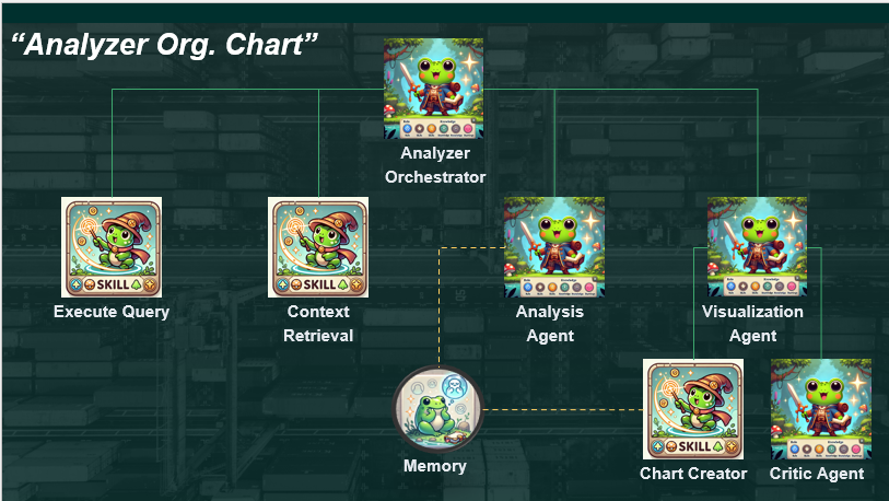
An agent is the intelligent layer that decides what to do. It's like a project manager who understands the goal, plans the approach, and uses available skills and tools to get the job done.

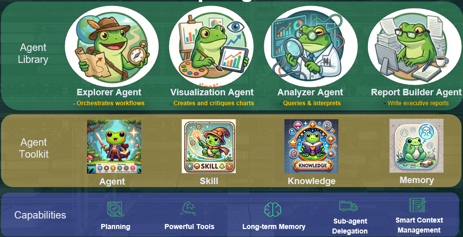
Note that not all these agents are exposed to users, in which case they are available as skills for other agents to use under the hood.

Agent Library

The Ada ecosystem includes many specialized agents (some of which are shown in the image above), each designed for specific analytical and reporting tasks.

Why specialization helps:

• ‍Higher reliability: narrower scope reduces ambiguity and improves tool choice.
• ‍Reusable expertise: prompts, skills, and knowledge can be tuned per domain.‍
• Parallelism and delegation: a coordinator agent can hand off sub-tasks to experts.‍
• Clearer governance: permissions can be scoped per agent (e.g., who can write files).

Agent Toolkit Framework

The agent toolkit is built on four foundational concepts that enable flexible and powerful agent development:

Agent

The core reasoning component - a large language model equipped with specialized skills and capabilities.

In addition to the model itself, an agent definition typically includes:

• Role and objective (what it is trying to accomplish)
• Constraints (what it must not do)
• Available skills/tools (its action space)
• Output contract (expected format, e.g., JSON, markdown report)
• Termination rules (when to stop vs. escalate)

Skill

A versatile building block that packages how to do something. This modularity allows agents to be composed and extended dynamically.

A skill may:

• Wrap a single tool,
• Orchestrate multiple tools in a workflow, or
• Delegate to another specialized agent.

Knowledge

A mechanism for injecting domain-specific expertise into agents at runtime, enabling them to operate effectively in specialized fields without requiring model retraining.

Memory

An intelligent storage system that helps agents overcome context-management challenges by preserving important information for future use, enabling continuity across interactions.

Core Capabilities

Current implementation supports several advanced capabilities enabled by the agent toolkit:

Planning

Agents can build structured plans that improve the accuracy and quality of final outputs through systematic decomposition of complex tasks.

Powerful Tools

The system supports custom tools provided by users, allowing agents to integrate with existing workflows and data infrastructure.

Long-term Memory

Persistent memory enables agents to maintain context and track important information across extended work sessions.

Sub-agent Delegation

Complex tasks can be delegated to specialized sub-agents, allowing for efficient division of labor and expertise application.

Smart Context Management

The system intelligently manages context to ensure agents have access to relevant information while avoiding context window limitations.

How They Work Together

Below is a simple workflow showing how different components work together. For simplicity, not all components are included here.

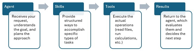
An agent is the intelligent layer that decides what to do. It's like a project manager who understands the goal, plans the approach, and uses available skills and tools to get the job done.

Skills are packaged capabilities that combine one or more tools with guidance on when and how to use them. Think of a skill as a trained procedure or technique.

Tools are the specific actions an AI agent can perform. They are specialized and do one specific thing reliably. They don't make decisions - they just execute when called.

Logs

As an AI Agent works, it produces the logs which include steps that the agent takes, tools it calls, as well as a work summary. The AI Response sections are typically the most useful as they explain the exploration plan, the work it has done, and the results after exploration. This is generally a response to the user. While all others are more for internal processes.

Example: Analyzer Agent

1. User submits data analysis request to the Analyzer Agent
2. Context Retrieval skill fetches relevant background information and helps determine relevant data tables
3. Execute Query skill retrieves and processes raw data
4. Analysis Agent synthesizes findings from results and provides recommendations. These are saved in Memory.
5. Visualization Agent creates charts using Chart Creator skill and Memory-informed context
6. Critic Agent reviews the charts to ensure that they answer user's questions and are formatted properly and suggests improvements
7. Final polished analysis and visualizations delivered to user

Other Helpful Resources

• Learn more about Cosmic Frog
• Learn more about DataStar
• Learn more about Ada
• The Modeler AI Agent
• The Model Output Insights AI Agent
• The Data Cleansing AI Agent
• The Data Profiler AI Agent

Introduction

Exciting tools that drastically shorten the time spent wrangling data, building supply chain models for Cosmic Frog, and analyzing outputs of these models are now available on the Optilogic platform.

Collectively, the Optilogic agentic AI tools are called Ada. This is after Ada Lovelace, widely regarded as the world’s first computer programmer and one of the earliest visionaries to recognize the potential of computational systems beyond pure calculation.

This documentation briefly explains how to access these AI Agents and Utilities, lists the available tools with a short description of each, and provides links to detailed documentation for several of these tools.

Helpful Resources

Before we dive into how to access the AI Agents & Utilities, here are a few links you may find helpful:

• Basic knowledge of DataStar and chatting with Ada is recommended. Start with:
  
  • The introductory video in the "Getting Started with DataStar: Application Overview" Help Center article.‍
  • The Getting Started with Ada & Agentic AI Help Center article.
• Please see the "AI Agents: Architecture and Components" Help Center article If you are interested in understanding how the Optilogic AI Agents work at a detailed level.
• These are the direct links to detailed documentation for several of the tools (they are also provided in the tools list in the last section):‍
  
  • Modeler AI Agent‍
  • Model Outputs Insights AI Agent‍
  • Data Cleansing AI Agent‍
  • Data Profiler AI Agent‍
  • Full Truckload Costing Utility‍
  • Less-Than-Truckload Costing Utility

Accessing Agents

Four of the available agents can be accessed by chatting with Ada and all of them can be accessed by using Run AI Agent tasks in DataStar.

Chat with Ada

When chatting with Ada on the next generation Optilogic platform, users can select the agent they want to use for their prompt:

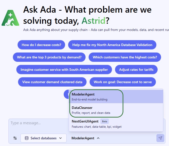
Please note that:

• The Modeler agent can use the Model Output Insights agent as a tool. Therefore, you can access the functionality of the Model Output Insights agent through the chat UI by selecting the Modeler Agent as the prompt's agent.
• Similarly, the Data Cleanser agent can use the Data Profiler agent as a tool. Therefore, you can access the functionality of the Data Profiler agent through the chat UI by selecting the Data Cleanser Agent as the prompt's agent.

Please refer to the detailed documentation on the individual agents and the getting started with Ada & Agentic AI article to learn more about using these when chatting with Ada.

DataStar

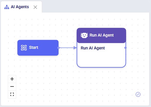
At a high level, the steps in DatsStar are as follows (screenshots follow beneath):

1. Open the DataStar application on the Optilogic platform
2. Create a new project in DataStar, see the "Creating Projects & Data Connections" section in the DataStar Overview documentation.
3. Create a new macro in the project.
4. From the Tasks tab on the right, drag and drop a Run AI Agent task onto the macro canvas.
5. In the configuration of the task, choose the Agent you want to use from the list in the Select Utility section.
6. Configure the Agent inputs in the Configure Utility section.
7. Optionally configure the Run Configuration and Notes sections.
8. Run the macro or just the Run AI Agent task by itself to execute the selected Agent.

Your macro canvas will look similar to the following screenshot after step #4:

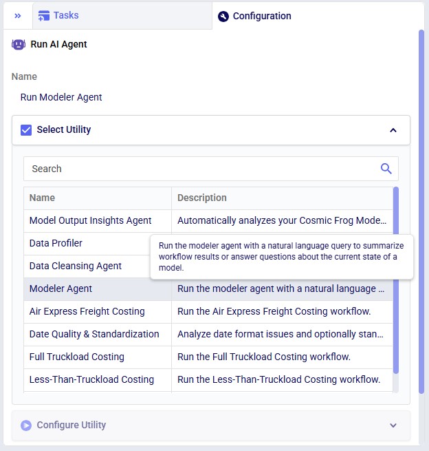
After adding a task, its configuration tab is automatically shown on the right-hand side. Give the task a name, and then select the Agent you want to use from the list of available Agents in the Select Utility section. You can also use the Search box to quickly find any Agent that contains certain text in its name or description. Hover over the description of an Agent to see the full description in case it is not entirely visible:

Once an Agent has been selected by clicking on it, the Configure Utility section becomes available. The inputs here will differ based on the Agent/Utility that has been selected. In the next screenshot the Configure Utility section of the Modeler Agent is shown:

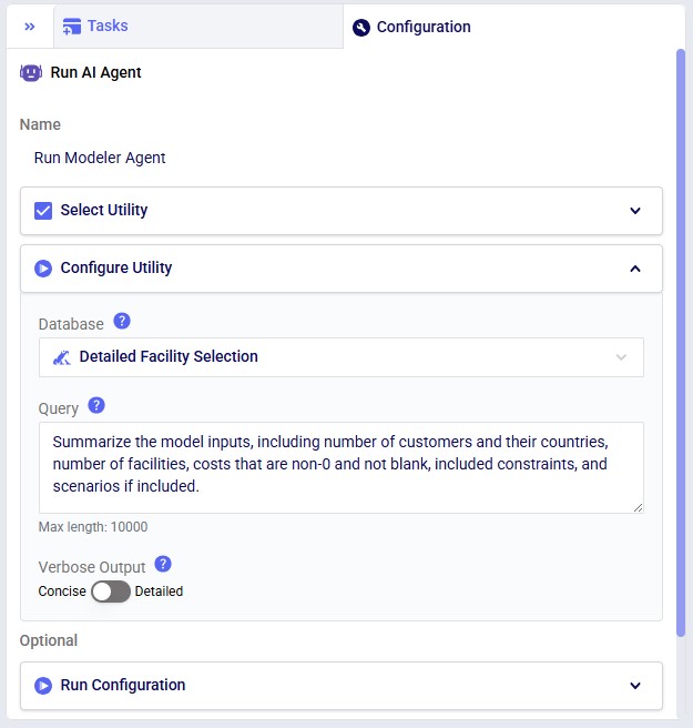
Provide the inputs for at least the required parameters, and if desired for any optional ones. Note that hovering over a blue question mark icon will bring up a hover box with a description of the parameter.

Accessing Utilities

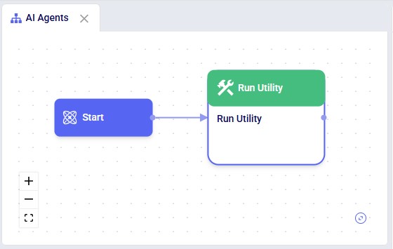
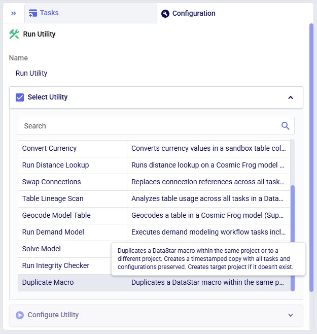
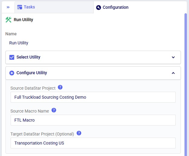
Using Utilities works in the same way as using AI Agents, just through the Run Utility task instead of the Run AI Agent task. The following 3 screenshots show 1) a Run Utility task added to a Macro, 2) its Select Utility section, and 3) the Configure Utility section of the Duplicate Macro utility:

Adjust Resource Size

Resource Size for both Run AI Agent and Run Utility tasks can be set in the Run Configuration section, which is indicated as optional. However, for most agents and utilities, the default 3XS Resource Size is not sufficient. It is recommended to update this to XS:

Available Agents & Utilities

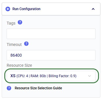
The folloing AI Agents and Utilities are currently available. More are being added as they come available. For each a short description is given and for those that have more detailed documentation to go with them, a link to this documentation is included.

AI Agents

• Model Output Insights Agent: Automatically analyzes your Cosmic Frog Model outputs and generates a report. Detailed documentation for this agent can be found here.
• Data Profiler: Run the full data profiler pipeline with statistical analysis, LLM-powered descriptions, quality scoring, alerts, and PK/FK discovery. Detailed documentation for this agent can be found here.‍
• Data Cleansing Agent: Run an AI-powered data cleansing agent with natural language prompts to intelligently analyze and fix data quality issues. Detailed documentation for this agent can be found here.‍
• Modeler Agent: Run the modeler agent with a natural language query to summarize workflow results or answer questions about the current state of the model. Detailed documentation for this agent can be found here.‍
• Air Express Freight Costing: Run the Air Express freight Costing workflow.Date Quality & Standardization: Analyze date format issues and optionally standardize dates to a target format.‍
• Full Truckload Costing: Run the Full Truckload Costing workflow. Detailed documentation for this agent can be found here.‍
• Less-Than-Truckload Costing: Run the Less-Than-Truckload Costing workflow. Detailed documentation for this agent can be found here.

Utilities

• Run Macro: Executes a DataStar macro in a specified project. Connects to the project, retrieves the macro, runs it, and waits for completion. Reports run status and errors if execution fails.
• Duplicate Task: Duplicates a DataStar task within the same macro or to a different macro. Creates a timestamped copy with all configurations preserved. Both target project and target macro must be provided together if specified. If target project and target macro are not specified, the task is copied to the same macro it exists in.
• Convert Data Guru Project into DataStar: Converts Data Guru logic documented in DG Documenter into DataStar. Reach out to support@optilogic.com for access to DG Documenter and for help migrating Data Guru to DataStar.
• Convert Currency: Converts currency values in a sandbox table column using current exchange rates. Creates a new column with converted values. Non-numeric values are saved as NaN. Requires storing a secret with key name 'DATASTAR_EXCHANGE_RATE_API_KEY' and value fetched from https://www.exchangerate-api.com/.
• Run Distance Lookup: Runs distance lookup on a Cosmic Frog model and stores distance records in the model's TransitMatrix table. Supports multiple geo providers (GreatCircle, PCMiler, Bing, Azure, OLRouting), configurable distance units, arc defining tables, and routing preferences.‍
• Swap Connections: Replaces connection references across all tasks in a DataStar project. Updates source/destination connections in Import/Export tasks and connection in RunSQL tasks. Validates connections exist and are the same type. Automatically updates table paths for file-based connections.
• Table Lineage Scan: Analyzes table usage across all tasks in a DataStar project. Categorizes usage as source (task reads from table), destination (task writes to table), or sql (table referenced in SQL query). Provides high-level summary and detailed task breakdown with execution order.‍
• Geocode Model Table: Geocodes a table in a Cosmic Frog model (Suppliers, Facilities, or Customers). Waits for completion and reports results by default. Supports fire-and-forget mode to skip waiting.‍
• Run Demand Model: Executes demand modeling workflow tasks including hierarchy generation, forecasting, and reconciliation. Supports CSV, Parquet, and DataStar adapters for flexible data I/O.
• Solve Model: Solves a Cosmic Frog model by running one or more scenarios. Runs all scenarios by default or a specified list. Supports custom engine, resource size, and infeasibility check options. Waits for completion and reports results.
• Run Integrity Checker: Runs integrity checker against a Cosmic Frog model and writes results to DataStar. Validates the entire model or a single table, then saves table errors, run metadata, and table status to the project's sandbox.
• Duplicate Macro: Duplicates a DataStar macro within the same project or to a different project. Creates a timestamped copy with all tasks and configurations preserved. Creates target project if it doesn't exist.

At Optilogic, we have built the next generation (next-gen) platform to complement our AI. It is a modern, unified workspace where users:

• Never lose their place: switch between applications like SQL Editor or Run manager without losing context
• Engage in a way that is natural to them, whether this is fully AI guided, using AI-as-copilot, or working heads-down in familiar tools
• Work in an environment that reduces clutter and only surfaces what matters: the platform grows with your session and persists where you left off
• Experience a cohesive framework that handles artifacts and iterative workflows seamlessly

While the next-gen platform is still in development, there is plenty available already for users to start working with it. Especially the AI-first approach will be a gamechanger for many. This documentation gives a high-level overview of the new platform. Please see the separate Getting Started with Ada & Agentic AI documentation for in-depth documentation on Ada, your supply chain modeling partner.

Logging in and First Time Configuration

Optilogic users can log into the next-gen platform at https://ai.optilogic.app, using the same credentials as those used to log into the current platform (on https://optilogic.app).

Once logged in, you are walked through 3 setup windows, shown in the following screenshots.

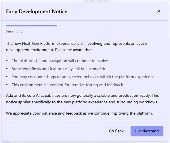
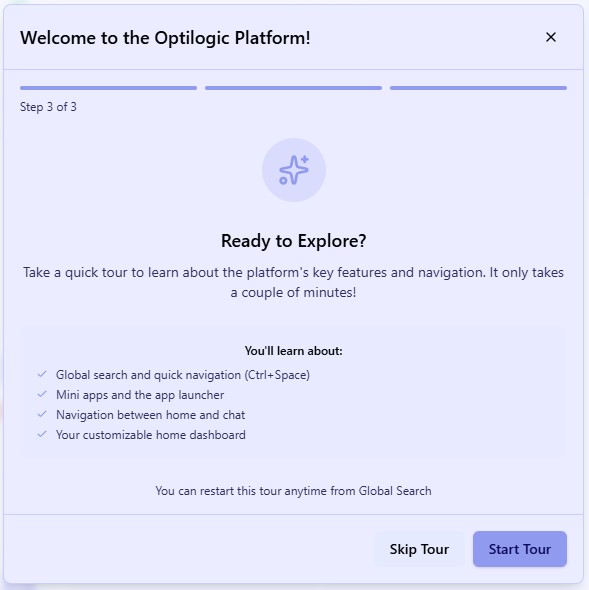
It is recommended to take the quick tour to learn about the platform. After it completes, you can follow another walkthrough, this one centered around using Ada through the chat UI. If you want to return to either of these tours later, you can find these in the Actions results part of Global Search (Ctrl + Space) after typing “introduction tour” or “Ada tour” in the search textbox.

Home Page and Sidebar

Your Home page will look similar to this:

1. In the top central part of the platform, Ada is available to immediately dive into any questions and tasks.
2. Further below, there are additional widgets, in this case a Recent Work one showing all recent DataStar and Cosmic Frog work and a Goals one for users to jump straight back in from where they left off.
3. The sidebar on the left provides quick access to all features.

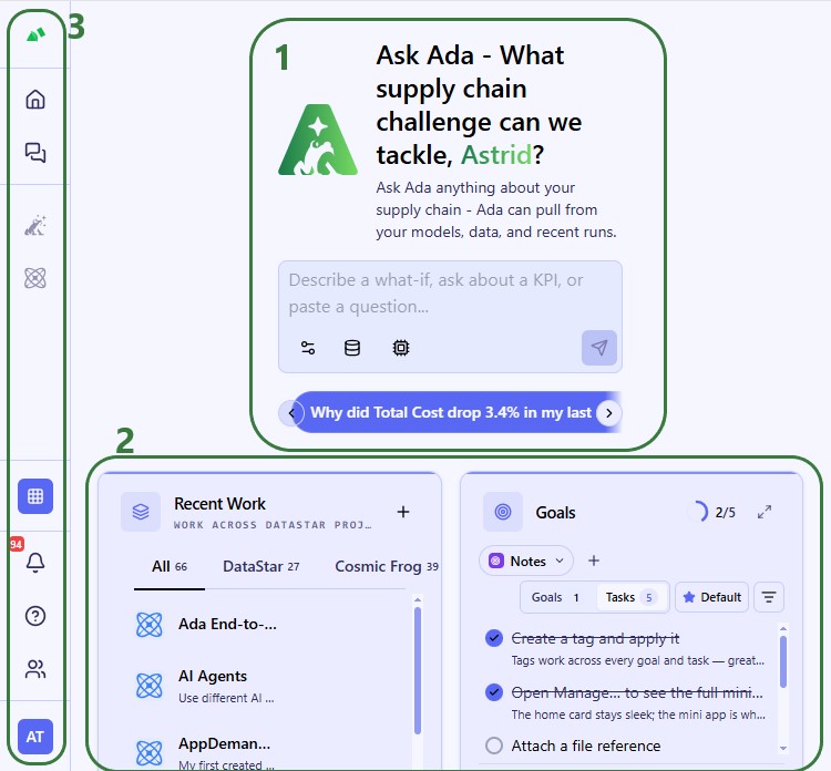
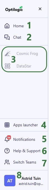
Clicking anywhere in the sidebar will expand it:

1. Click on Home to return to the home page as shown in the previous screenshot.
2. Click on Chat to open the chat UI full screen, including historical conversations with Ada.
3. In this area, applications that have been opened will be added to the rail, like a taskbar with open applications. Note that:
   1. Cosmic Frog and DataStar are by default pinned here as these are the most used Optilogic applications. They are greyed out when not open; click on them to open the application.
   2. Use the Apps launcher (next bullet) to open other applications.
   3. Applications can be active multiple times, e.g. 2 instances of Lightning Editor can be active showing 2 different files, see also the next section.
   4. Right-clicking on an application brings up a context menu, see also the next section.
4. The Apps Launcher can be used to open any of the Optilogic applications, but also to do a global search through files, databases, settings, and tours. Use the Ctrl + Space shortcut to open the Apps Launcher/Global Search at any time. See also the Apps Launcher section further below.
5. When activity happens within your Optilogic account, notifications alert you to this. This includes notifications for Cosmic Frog model and scenario runs, utilizing geocoding or the Integrity Checker within Cosmic Frog, DataStar Macro runs, database archival, and more. See also the Notifications section further below.
6. Click on Help & Support to easily access several helpful resources, use the AI Help Guide or to contact Optilogic support. This Help & Support window can also be brought up by using the F1 function key. See also the Help & Support section further below.
7. Use the Switch Teams option to change context between your own account (“My Account”) and any teams you may be part of. See Getting Started with Optilogic Teams for more information on using the Teams features. See also the Switch Teams section below.
8. Access your account settings by clicking on your profile picture. These include items like settings, preferences, and signing out. See also the Account Settings section further below.

Applications Added to the Taskbar

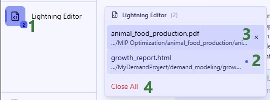
When an application has been opened, it is added to the taskbar. If multiple instances of it are active, we can see that too:

1. The Lightning Editor is showing in the taskbar, the 2 at the right bottom of the icon indicates that 2 instances of this application are active.
2. Hovering over the Lightning Editor icon in the taskbar brings up the list of active instances. The 1 that is open and showing in the UI, by default to the right-hand side of the Home page or Ada chat, is indicated with a blue dot to the right.
3. Hovering over an instance in the list of active instances shows the close button to close that specific instance.
4. At the bottom of the list, a Close All button is available to close all instances of the Lightning Editor with one click.

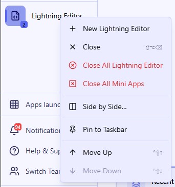
A context-menu is also available when right-clicking on applications added to the taskbar:

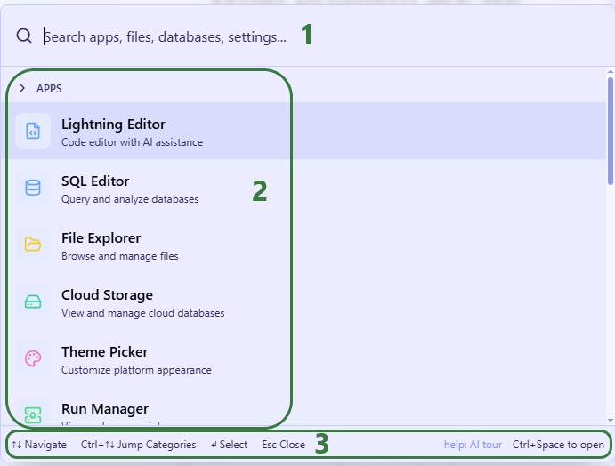
From top to bottom:

1. Open another instance of this application, in this case of the Lightning Editor.
2. Close the oldest instance of this application.
3. Close all instances of this application.
4. Close all active applications in the taskbar.
5. Use Side by Side… to see this application next to another. Choosing this option opens the Apps Launcher where you can choose what to show next to this application.
6. Pin the application to the taskbar, it will then be shown in the part of the sidebar just above (with Cosmic Frog and DataStar), so it can be opened from there immediately. If an application is already pinned to the taskbar, this option changes to Unpin from Taskbar.
7. Use Move Up and Move Down to change the position of the application in the taskbar.

Apps Launcher

The following modal comes up when clicking on the Apps Launcher in the sidebar:

1. Use the search textbox to find applications, databases, settings, tours, etc.
2. At the top of the list, all available applications are listed.
3. Shortcuts on how to scroll through the list are shown at the bottom.

Notifications

When clicking on Notifications in the sidebar, the notifications list will open up on the right-hand side of the platform, next to the Home page or active chat with Ada:

1. Use these buttons to, respectively, make the Notifications app full screen, pop it out to a new window, minimize it, or close it.
2. Here, the number of notifications is shown, users can toggle between showing only unread ones or showing all, and under the 3 horizontal dots button 2 additional options to mark all messages as read and to delete all messages are available.
3. By default, all notifications are shown; users can switch to Active view to only show notifications of processes which are currently in progress.
4. For each notification, there is a card which indicates the type of notification, status, and when this activity happened.
5. For notifications of activities that are listed in the Run Manager application’s job list, this View Progress option is available. It opens the job in the Run Manager application.

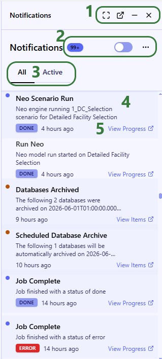
It is not shown in the screenshot, but hovering over a Notification card will bring up a checkmark icon and an x icon which can be used to mark the notification as read and to close it.

Help & Support

Clicking on Help & Support in the sidebar brings up the following modal:

1. Clicking on Contact Support brings up a window where you can write a message to the Optilogic Support team, attach databases/files to it, and submit it.
2. In the AI Help Guide textbox write what you need help with, and it will create a guided tour for you.
3. The Resources part links out to:
   1. The Knowledge Library in Optilogic’s online Help Center
   2. The Frogger Pond Community where Optilogic users can connect with and learn from each other and Optilogic experts
   3. The Optilogic contact us page where you can send a message to arrange a meeting
   4. The Live & On-Demand Training website which has a wide offering of training resources

Switch Teams

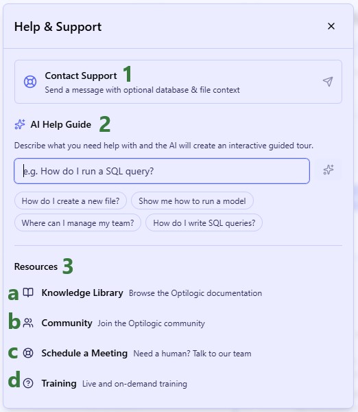
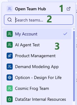
If your organization uses the Teams set of features, you can easily switch teams by clicking on the Switch Teams button:

1. If you want to open the Team Hub application, click on the icon at the right top, which will open it within the platform on the right-hand side.
2. You can quickly find the team you want to switch to by typing part of its name in the Search box.
3. The list of teams the user is part of is shown here; the workspace the user is currently using is indicated by the checkmark.

Account Settings

Configure your account by using the options found when clicking on your profile picture:

1. Click on your profile picture/initials to bring up all options.
2. Clicking on Profile will open the Profile menu on the right-hand side of the platform. Under Profile you can access:
   1. Overview – username, email, password and a high-level summary of the account.
   2. App Keys – these are used to establish a secure connection to the Optilogic platform and can be created and managed here.
   3. Secrets – may be needed to run certain utilities and can be created here.
   4. Geo Provider Keys – if you have a key for a geocoding provider (Mapbox, Google, Bing, PTV, PC Miler, or Azure Maps), you can enter it here so that the provider will be used for geocoding and distance calculations within Cosmic Frog.
   5. Subscription – review subscription options and payment details.
   6. Usage – shows the usage over time of the current Team the user is in. You can adjust the time window and granularity. Optionally, download your usage information in a CSV file.
   7. Firewall Rules – rules can be created and managed here for allowing certain IP addresses/ranges access.
3. Clicking on Settings will open the Settings menu on the right-hand side of the platform. Under Settings you can access and configure:
   1. Notifications – enable/disable push notifications and further configure the level and type of notifications under advanced settings.
   2. Apps – set the default app for opening databases, whether autosave is on in Lightning Editor, the order your apps appear in on the sidebar, and manage run configuration settings.
   3. Labs – set whether models can be run from anywhere in the platform and enable/disable access to run summaries.
   4. Test / Stub settings – choose the location for the applications icon rail (left (default), or right), the location in the platform where apps will open (right (default), or left), and your layout mode (auto (default), mobile, or desktop).
4. Clicking on REST API opens a new browser tab with the documentation on Optilogic’s REST API.
5. Clicking on Downloads opens the Downloads application on the right-hand side of the platform – any files ready for download and previously downloaded will be listed here.
6. What’s New - find the latest Release Notes for Optilogic applications here.
7. Click on Logout to sign out of the next-gen Optilogic platform.

Open Applications

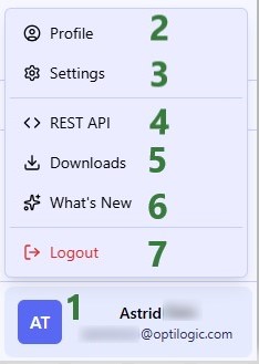
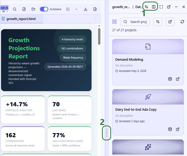
As mentioned under bullet 3d just above, by default, applications will be opened on the right-hand side of the screen next to either the homepage or chat with Ada page:

1. When you hover over the line in between the app and home/chat (to the left, not shown), the cursor will change to 2 arrows pointing away from each other, clicking the mouse and dragging left or right will resize the app area.
2. When applications are open, options are available at the top right to, respectively: open another application side by side, open the application full screen (no home/chat), enter Agentic mode, pop the application out into a new window, minimize the application (but keep it on the taskbar), or close the application (remove it from the taskbar). Depending on the application that is open, only a subset of these may be available.

Side by Side

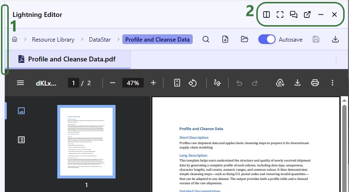
When you enter side by side mode, the second application will be shown to the left of the first, taking the place of home/chat. Here, first DataStar was opened and then Lightning Editor by using the Side by Side option:

1. The options here allow the user to swap the position of the 2 applications that are open side by side and to exit side by side mode which will close the application that was opened second.
2. Click on and drag the line in between the applications to resize them.

Cosmic Frog

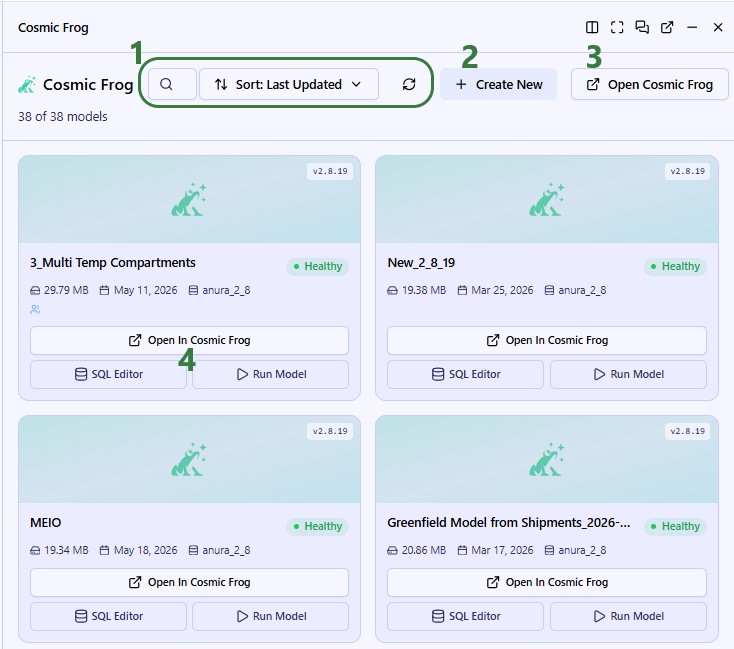
Whilst Cosmic Frog is not yet entirely integrated into the next-gen platform, users can open it, see their model list, and run scenarios from here:

1. Options to search in the model list and to sort it in different ways are available at the top.
2. Users can create a new Cosmic Frog model by using this Create New button.
3. To open Cosmic Frog in a new browser tab in the current platform, click on Open Cosmic Frog.
4. A model card gives basic information about the model and allows a user to open it in Cosmic Frog in the current platform in a new browser tab, to open it in SQL Editor within the next-gen platform, or to run the model.

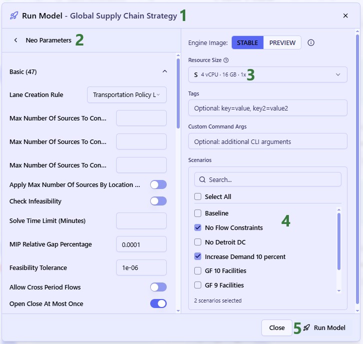
When clicking on Run Model for one of the available models, the following modal comes up:

2. The Run Model modal for the selected model, Global Supply Chain Strategy in our example.
3. In the previous step (not shown), we have chosen Neo as the engine to use for our scenario runs, and therefore the Neo Parameters are shown here now. Make any adjustments to them as needed. For an explanation of the technology parameters for all engines, please see Running Models & Scenarios in Cosmic Frog.
4. Set the Resource Size for your runs. For guidance, please see the Resource Size Selection Guidance Help Center article.
5. Select the scenario(s) to run.
6. Click on Run Model to kick off the scenario(s). Alternatively, click on Close if choosing to not go ahead with any runs.

DataStar

DataStar is also not yet entirely integrated, but projects, macros, and connections can be viewed and macros can be run:

1. Options to search in the project list and to sort it in different ways are available at the top.
2. To open DataStar in a new browser tab in the current platform, click on Open DataStar.
3. Clicking on a project card will open it within the next-gen platform, see next screenshot.
4. Options to open the DataStar project database in SQL Editor and to open it in DataStar in the current platform in a new browser tab are available from the project card.

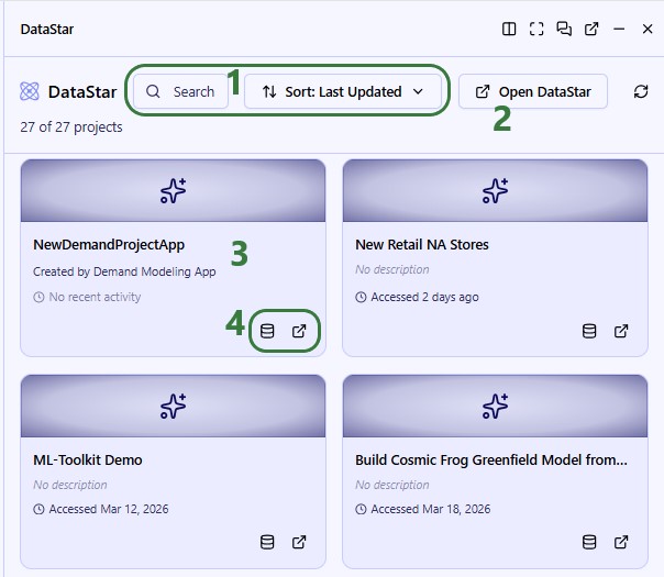
The user clicks on the New Retail NA Stores project card to open it:

1. At the top, it is indicated that the project of this name is now open.
2. We can choose to see the Macros, Runs, Connectors, and an Overview of this DataStar project.
3. We are looking at the Macros in this project and see that 1 is present. It is named Import New NA Customers and was last run 3 days ago. Clicking on it will open the Macro, see next screenshot.

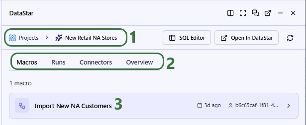
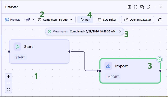
We have clicked on the Import New NA Customers to open it:

1. The Macro Canvas is now open, showing the simple macro which only has 1 Import task.
2. From the runs drop-down list, users can choose to see the results of this macro’s past and ongoing runs.
3. The run that was picked was executed on 5/29/2026 and it completed successfully. We can also see this from the task on the Macro Canvas: it has a green outline and green checkmark at the right top.
4. To run the macro, click on the Run button.

Next Gen UI Agent

The Next Gen UI Agent is one of Ada’s agents and can be accessed through the chat UI. It can help you with anything UI/platform related, like finding things within the platform, creating charts/tables, reporting on KPIs, and guidance on widget creation/removal.

1. When you are in the chat part of the platform, first select the database(s) you want your prompt to use (if any). This can be 1 or multiple Cosmic Frog models, DataStar projects, or Postgres databases.
2. From the agents drop-down list, select the Next Gen UI Agent.
3. Enter your prompt. Here, we have asked the agent to create a stacked bar chart by scenario from cost outputs located in the Optimization Network Summary output table of the connected database (a Cosmic Frog model named Global Supply Chain Strategy, which is available from the Resource Library).

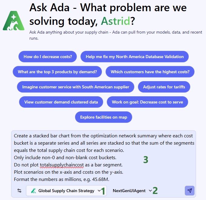
The response to the prompt is as follows, where at the top the asked for bar chart is shown and the agent proactively added the data used for the chart in a table underneath the chart:

Example Prompts

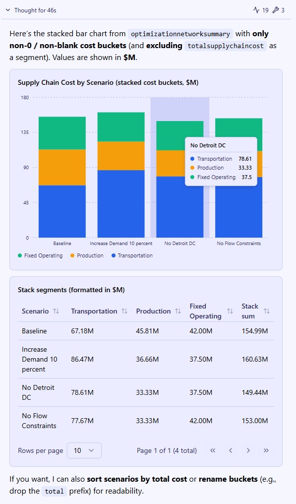
Here are a few example prompts you can try using the Next Gen UI Agent:

• Can you create a chart showing total cost and total revenue for all scenarios in the connected Cosmic Frog model (table Optimization Network Summary, Total Supply Chain Cost and Total Revenue columns)?
• Can you create a guided tour on how to find a particular PDF file and view it in the platform?
• What are the statistics of my 50 most recent jobs?
• Add “Review new historical productions file” to my tasks.
• What can this agent help me with?
• Can you help me re-phrase my prompt to achieve X?

Other Helpful Resources

• Learn more about Ada & Agentic AI
• Learn more about Cosmic Frog‍
• Learn more about DataStar

As always, please reach out to Optilogic Support (support@optilogic.com) in case of questions or feedback.

In just a few clicks, you can create a free account on the Optilogic platform, which includes Cosmic Frog and DataStar among other applications. This document walks you through the steps.

Quick Start (2-3 minutes)

If you just want the fastest way to get started:

1. Go to the Optilogic Create Account page
2. Enter your name, email, and phone number
3. Click Next Step
4. Choose one:
   • Sign in with Google, Microsoft, or LinkedIn (fastest)
   • OR create a password
5. Complete the form and click Submit
6. Check your email and click Verify Email
7. Answer a few setup questions → you're in!

‍

Overview of the Sign-Up Process

You will go through 3 main stages:

1. Enter basic details
2. Choose sign-in method (SSO or email/password)
3. Verify email and finish setup

Start the Account Sign-up

To start, go to the Create a Free Account page on Optilogic's website. You will see the following form on the right-hand side:

1. Fill out your name, email address and phone number in the personal details section.
2. Optionally, tick the boxes for receiving a call to discuss your objectives and receiving latest information from Optilogic. By default, these are unchecked.
3. Click on the Next Step button to continue the account creation process.
4. In case you will be using the Optilogic platform in an academic setting, you can instead click on the link to create an education account.

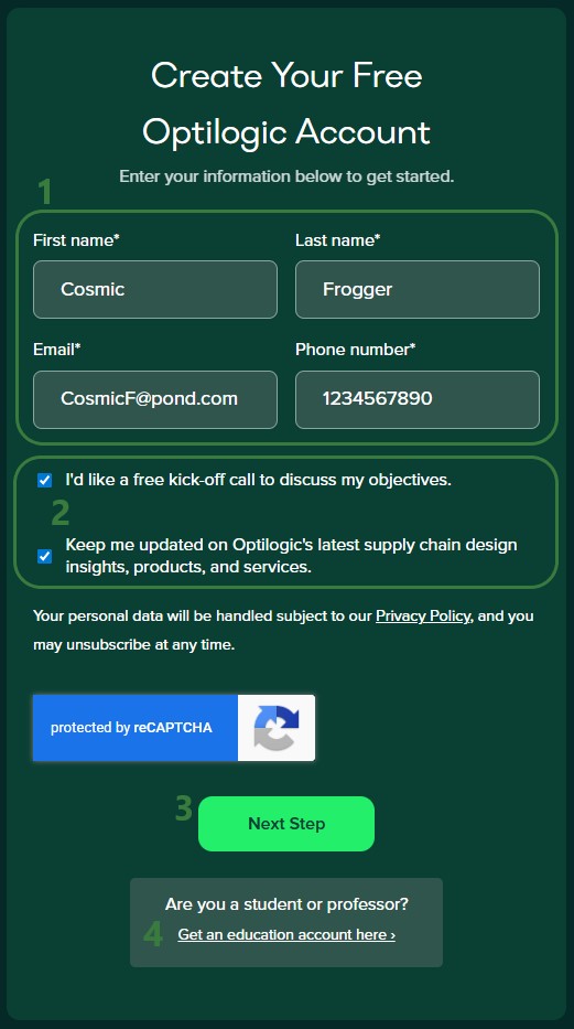
After clicking on the Next Step button, the form changes to the following message. In addition, a new browser tab has been opened and has automatically become the active tab (see screenshot below this one):

The new active tab shows the following Create An Account form:

1. At the top, 3 Single Sign-On (SSO) options are available. If you have SSO enabled for Microsoft, Google or LinkedIn and you wish to use it for logging into the Optilogic platform, then click on one of these options.
2. If you wish to use your email and a password to sign up, click on this option.

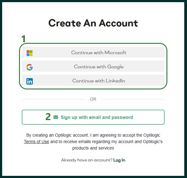
We will first go through the Single Sign-On steps using Google as the example in the next section. In the section after, Email and Password Steps, we will cover the email and password sign-up option.

Single Sign-On Steps

We will illustrate the single sign-on process by going through the steps using a Google account. These steps are similar when using a Microsoft or LinkedIn account.

First, you will be prompted which Google account you want to use. The one you are currently logged into will be listed and you can click on it to select it. If you want to use another Google account, click on the "Use another account" option.

‍

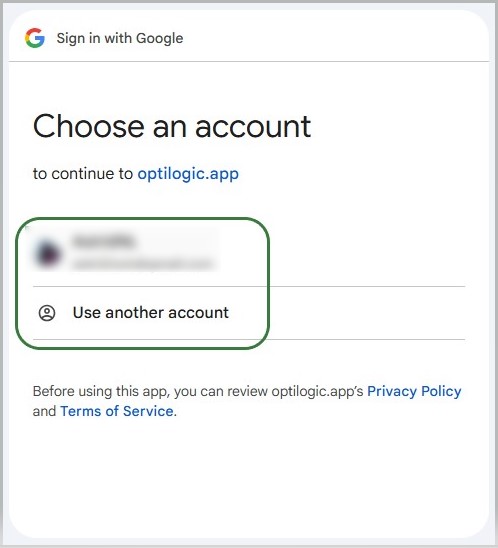
After selecting the Google account to use, the following form will appear:

1. The drop-down shows which Google account you are using. Click on it to go back to the previous step and select a different account.
2. The information that will be shared from Google with the Optilogic platform is listed here.
3. Click on the Continue button to go to the next step or click on the Cancel button to abort the sign-up using this SSO method.

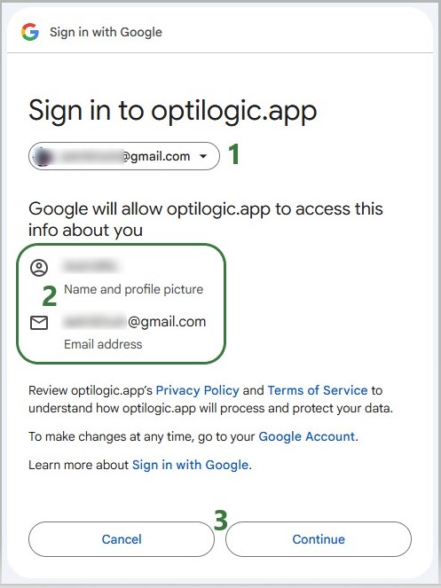
If you have clicked on the Continue button, the following form with user account information will come up. If any details are missing, please fill them out and then click on the Submit button.

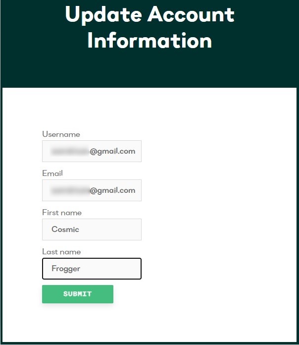
You have now signed up for an Optilogic account. The next step is to verify your email address, see the Verify Email and Configure Account section further below (link).

Email and Password Steps

If you have chosen the option to sign-up using your email address and a password, the bottom part of the sign-up form will now look as follows:

1. Fill out the credentials you will be using to login to the Optilogic platform.
2. Enter your personal info.
3. Click on the Submit button.

‍

Verify Email and Configure Account

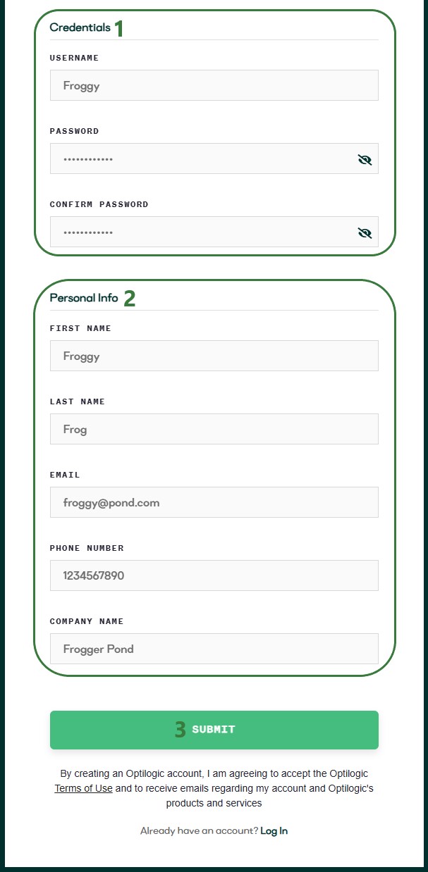
Regardless of if you used an SSO method or the username & password option to sign-up for an Optilogic account, the next steps are the same. After clicking on the Submit button, the following message will appear:

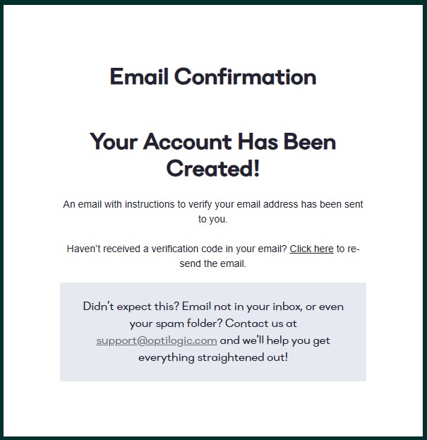
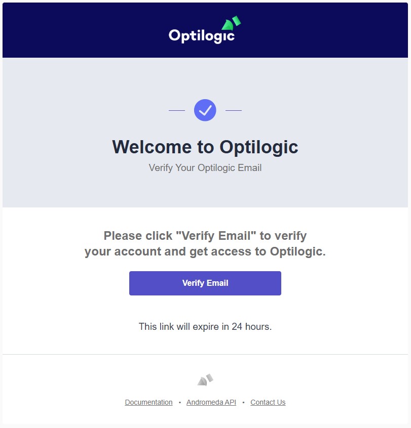
Go into your email account and find the email from Optilogic Support with the subject Verify Your Optilogic Email. In there, click on the Verify Email button:

‍

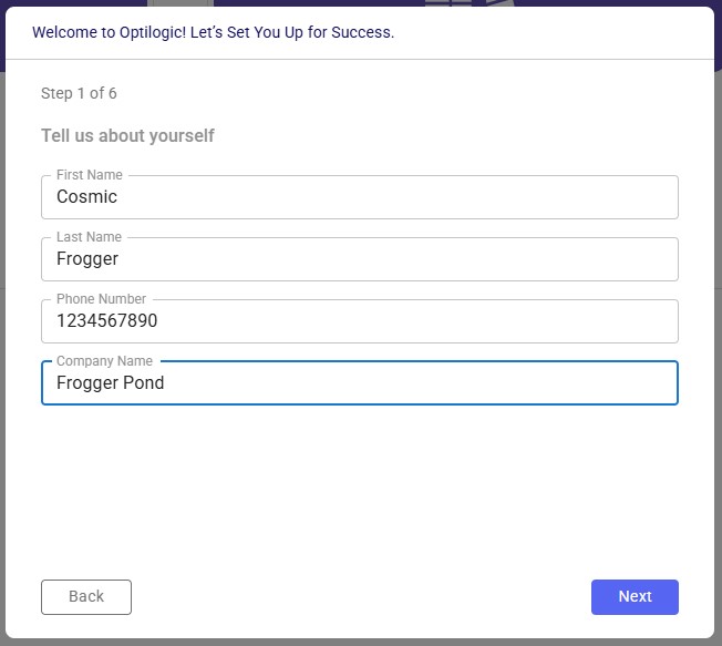
This will take you into the Optilogic platform, where you will be walked through a few quick questions to finalize your details and set up your account. Step 1 is pre-populated from your previous entries; if any are missing, please add them and then click on the Next button:

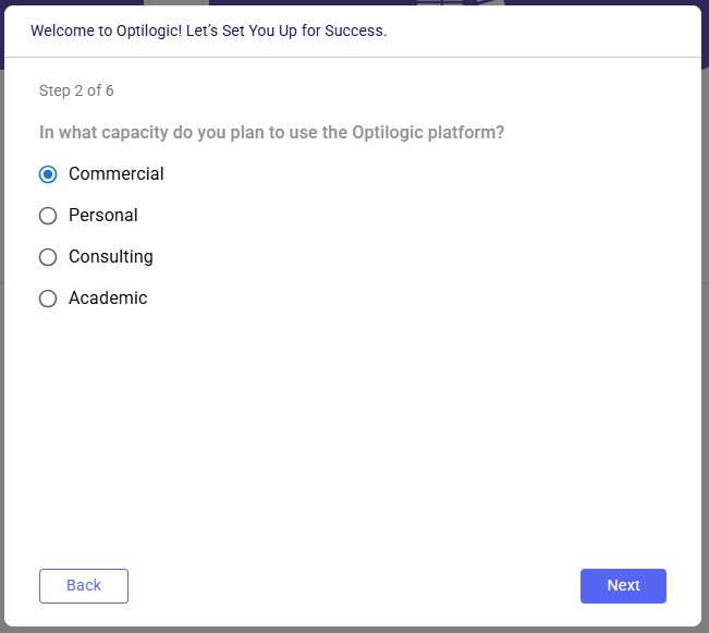
The next steps gather a bit more information:

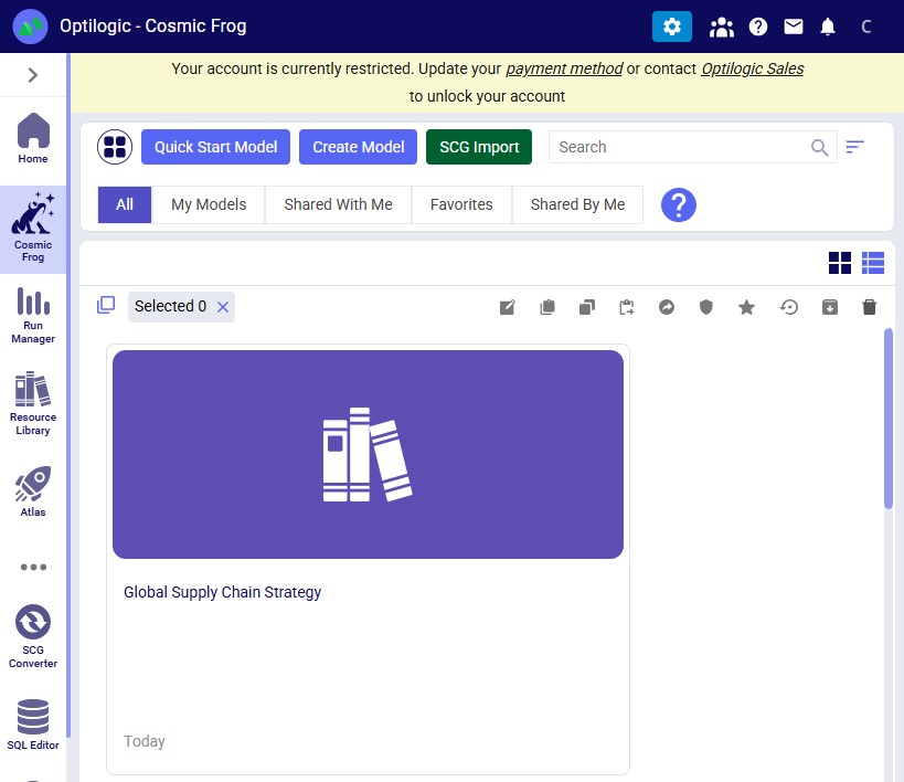
When completed, the Cosmic Frog application will be opened, and you can start exploring any of the 3 example models shown on the start page:

🎉 You're ready to start using Optilogic!

Sign-up for Account from Optilogic Login Page

Note that you can also sign up for an Optilogic account from the platform's login page (https://optilogic.app) by clicking on the Sign-Up link at the bottom. The options and steps are the same as documented above.

Troubleshooting

Did not receive verification email?

• Check spam/junk folder
• Wait a few minutes and try again
• Follow the steps in the Trouble Receiving Account Confirmation Email article

Wrong SSO account selected?

• Log out and restart the sign-up process

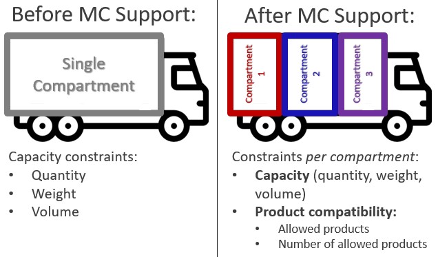
The Multiple Compartments (MC) feature allows a single transportation asset (e.g., truck, trailer) to be divided into independent compartments, each with its own capacity and compatibility constraints. This enables Hopper to produce more accurate, feasible, and operationally realistic transportation plans.

‍

Quick Start

Get up and running in 4 steps:

1. Define compartments - in the Compartment Configurations table, add one row per compartment. Give all rows of one configuration the same Compartment Configuration Name.
2. Link to asset - in the Transportation Assets table, set the Compartment Configuration Name field to your configuration name.
3. Run Hopper - Hopper now automatically enforces per-compartment capacity and compatibility rules.
4. Review output - check the Compartment Name column in the Transportation Optimization Shipment Summary output to see which compartment each shipment is assigned to.

‍

When to Use Multiple Compartments

Use this feature when one or more of your transportation assets have physically separate sections that must be loaded independently. Common examples:

• Tankers with separate liquid chambers (e.g., different fuel grades)
• Multi-temperature trucks with frozen, chilled, and ambient zones
• Segmented trailers where sections have different weight or volume limits

Without Multiple Compartments, Hopper checks only that the total shipment fits the total asset capacity. This can produce plans that look valid in the optimizer but cannot be executed operationally because individual compartments are overloaded or contain incompatible products.

How to configure Multiple Compartments

Three changes have been made to Hopper's data model: one new input table, one new field on an existing input table, and one new field on an existing output table.

Input Table: Compartment Configurations (new)

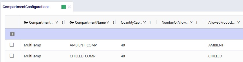
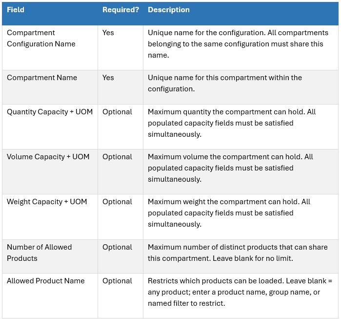
This table defines the structure and rules of the compartments that make up each configuration. Add one row per compartment; rows with the same Compartment Configuration Name form a single configuration.

‍

‍

Input Field: Compartment Configuration Name (Transportation Assets Table)

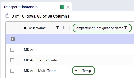
A new Compartment Configuration Name field has been added to the Transportation Assets table. Populate it with the name of a configuration defined in the Compartment Configurations table to enable compartment-level modeling for that asset.

Effect on Hopper's solver:

• Without a value (blank): Hopper uses single-capacity validation (total shipment <= total asset capacity).
• With a value: Hopper switches to compartment-level assignment and validates each compartment's constraints individually.

Output Field: Compartment Name (Transportation Shipment Summary Table)

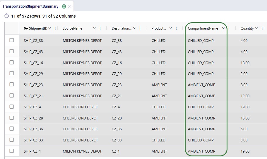
The Transportation Optimization Shipment Summary output table now includes a Compartment Name column. For any shipment transported on a multi-compartment asset, this column shows which compartment it was assigned to.

‍

This field enables:

• Operational validation - confirm physical loading assignments before execution
• Warehouse and loading-dock planning - sequence picking by compartment
• Compliance checks - verify product segregation rules are respected

Example: Single Compartment vs. Multiple Compartments

The following example runs two scenarios with the same "MK Artic Multi Temp" asset to illustrate the difference:

• Scenario A - Single Compartment: The asset has one pool with a maximum of 80 units total.
• Scenario B - Two Compartments (MultiTemp): The same asset uses the MultiTemp configuration - two compartments of 40 units each, one restricted to AMBIENT product and one to CHILLED product.

Both scenarios have other single-compartment assets available. In each scenario, the MK Artic Multi Temp asset is used for one route. The charts below show how much of each product is on board at each stop along that route (stops are ordered by route sequence on the x-axis; the asset is loaded at Milton Keynes and Chelmsford depots and delivers to the CZ locations).

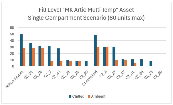
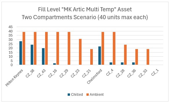
Key observations:

• Scenario A allows CHILLED to exceed 40 units on two segments - this would be physically impossible if those zones are separate compartments, meaning the plan cannot be executed as generated.
• Scenario B respects both compartment limits throughout the entire route.
• Scenario A delivers more product (150 vs. 109 units) to more customers (14 vs. 11) on this route - but only because it is ignoring real physical constraints.

‍

Summary

Multiple Compartments moves Hopper from aggregate capacity modeling to granular compartment-level modeling. This means:

• Each shipment is assigned to a specific compartment, not just a total pool
• Capacity, weight, volume, and product-compatibility rules are enforced per compartment
• Output plans reflect operational reality and can be executed without manual adjustment

Questions? Contact the Optilogic support team at support@optilogic.com.

Showing supply chains on maps is a great way to visualize them, to understand differences between scenarios, and to show how they evolve over time. Cosmic Frog offers users many configuration options to customize maps to their exact needs and compare them side-by-side. In this documentation we will cover how to create and configure maps in Cosmic Frog.

Maps Basics

In Cosmic Frog, a map represents a single geographic visualization composed of different layers. A layer is an individual supply chain element such as a customer, product flow, or facility. To show locations on a map, these need to exist in the master tables (e.g. Customers, Facilities, and Suppliers) and they need to have been geocoded (see also the How to Geocode Locations section in this help center article). Flow based layers are based on output tables, such as the OptimizationFlowSummary or SimulationFlowSummary and to draw these, the model needs to have been run so outputs are present in these output tables.

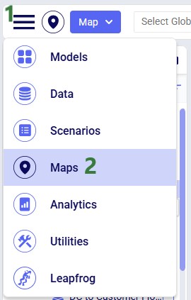
Maps can be accessed through the Maps module in Cosmic Frog:

1. Click on the Module menu at the top left in Cosmic Frog.
2. Choose Maps from the drop-down menu.

The Maps module opens and shows the first map in the Maps list; this will be the default pre-configured “Supply Chain” map for maps the user created and most models copied from the Resource Library:

1. The list of pre-configured maps and their layers is located on the left-hand side of the map, the next screenshot will cover this list in more detail.
2. The pre-configured Supply Chain map is showing by default when first opening the Maps module. Here, Customers are shown as small green circles (there are around 1.3k customers in this model), 7 Distribution Centers (DCs) are shown using a blue truck icon, 2 Factories are depicted with a blue building icon, and 2 Ports with an orange ship icon.
3. At the right top of a map, user will find following 4 map controls, from top to bottom:
   
   1. Enter fullscreen: clicking on this icon will maximize the map on the whole computer screen. Clicking on this icon again, which at that point will have the arrows pointing inwards, will exit fullscreen mode.
   2. Zoom in: clicking on this icon will zoom the map in. The map area will be used to show a smaller part of the world, and the features will become more detailed (e.g. smaller roads and smaller localities will become visible) as user zooms in more. Note that users can also zoom in using the scroll button on a mouse or putting two fingers on a mouse trackpad and moving them away from each other.
   3. Zoom out: clicking on this icon will zoom the map out. The map area will be used to show a larger part of the world and features will become less detailed. Note that users can also zoom out using the scroll button on a mouse or putting two fingers on a mouse trackpad and moving them closer to each other.
   4. Reset bearing to north: when working with a map, they may get moved so that the orientation is not the standard of top being north, right being east, etc. Click on this icon to reset the map so that the middle top part of the map faces north again.
4. Optionally, a Map Legend which can be configured by the user can be shown on the map. This will be covered in the Map Legend section further below.
5. Basic map and layer operations are available from the Map drop-down menu. See the Basic Map & Layer Operations section for more details.
6. The user can either set which scenario a map should use for each map individually (see the Map Filters section on how to do this) or they can use this Global Scenario Filter to set one scenario to be used by all Maps contained in the model. This filter is discussed in the Global Scenario Filter section further below.

Mouse Actions on Maps

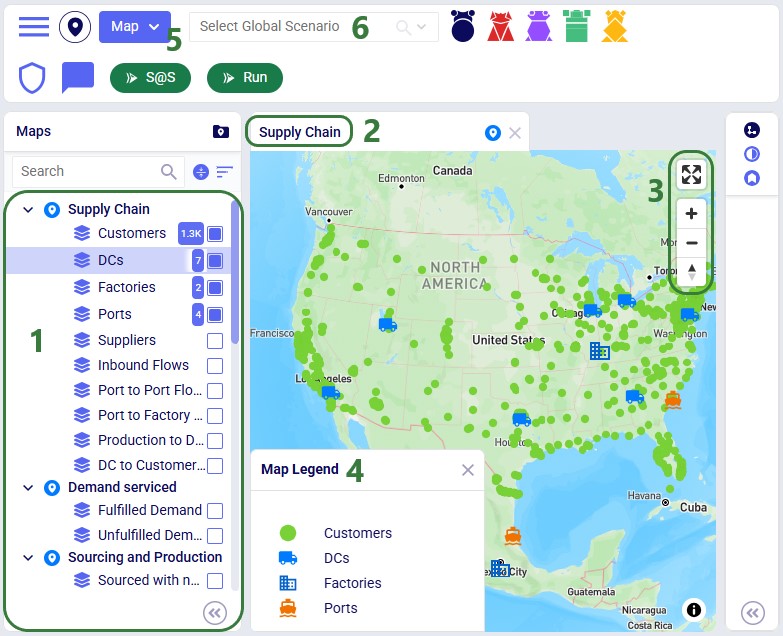
In addition to what is mentioned under bullet 4 of the screenshot just above, users can also perform following actions on maps:

• Users can drag the map to move it around to see a different part of the world: when hovering above the map with the mouse, the cursor becomes a hand. Click the mouse down and hold it down while you move in any direction to move the map.
• Shift and use left mouse / mouse trackpad to draw a marquee to zoom.
• To show a more 3-dimensional view where you can look down a street instead of looking at it from above: zoom in quite far, then hold CTRL down whilst using your left mouse button / track pad to tilt the projection:

• Following shortcuts for zooming, panning, and rotating are also available:
  
  • ‍‍= or +: increase the zoom level by 1
  • - or _: decrease the zoom level by 1
  • Shift and = or +: increase the zoom level by 2
  • Shift and – or _: decrease the zoom level by 2
  • Arrow keys: pan by 100 pixels
  • Shift and right arrow: increase the rotation by 15 degrees
  • Shift and left arrow: decrease the rotation by 15 degrees
  • Shift and up arrow: increase the pitch by 10 degrees
  • Shift and down arrow: decrease the pitch by 10 degrees

Maps List

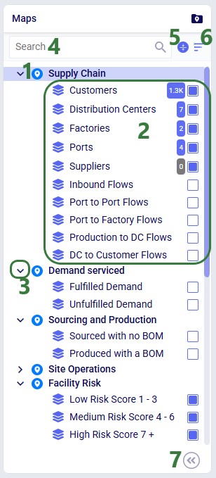
As we have seen in the screenshot above, the Maps module opens with a list of pre-configured maps and layers on the left-hand side:

1. The map named “Supply Chain” is selected in the list. When clicking on a map, it will be opened, and it becomes the active map.
2. This map has 10 layers. Five of the layers are enabled and will be showing on the map: Customers, Distribution Centers (renamed from Facilities), Factories, Ports, and Suppliers. Please note that:
   
   1. By default, only 3 layers (Customers, Facilities, and Suppliers) are enabled; the user has in addition enabled the Factories and Ports layers in this case.
   2. The number of records from the input or output table that is used to draw the layer is listed in a blue square to the left of its checkbox. If there are no records in the table used to draw the layer, then the square’s color is grey so users can easily identify these. This number of records reflects filtering the table based on the scenario, product(s), and period(s) the user has selected to show on the map (for more details, see the Map Filters and Maps of Multi-period Models sections further below). In addition, the number also reflects if user has filtered the table based on applying any filtering condition(s) or named filter(s) to the map layer (for more details, see the Condition Builder section further below).
   3. Map layers can be dragged to change the order of how they are drawn on the map:
      
      1. Layers that show locations (layer Type = Point) are always drawn on top of layers that show flows (layer Type = Line).
      2. Multiple layers of the same type are drawn on the map in the order they are listed (top to bottom), so drag any layer that should not be obscured by another layer below the layers it should be on top of.
3. Users can click on the chevron icon to collapse a map so that its layers are not visible in the list anymore. When collapsed, clicking on the chevron icon again will expand the map again and the layers become visible in the list. In the screenshot, all maps are expanded, except for the Site Operations map, which is collapsed.
4. At the top of the list users can free type text in a search box. This will filter the list of maps down to the maps where the map name or any of its layer names contain the text.
5. Clicking on this icon will collapse all maps, so that no layers are visible in the list, only the map names. Clicking on the icon again will expand all maps and all map layers become visible again.
6. Users can sort the maps in 2 ways that will be available when clicking on this icon:
   
   1. Default: the pre-configured maps are listed first and any maps added by the user are listed below in the order they were added.
   2. A-Z Name: this sorts the list in alphabetical order of map names. Clicking on the A-Z Name sort order icon again will sort them in reverse alphabetical order.
7. Click on this icon with 2 less than signs to hide the pane with the Maps list. The icon then turns into 2 greater than signs, which when clicked on will open the Maps list pane up again.

Basic Map & Layer Operations

The Map menu in the toolbar at the top of the Maps module allows users to perform basic map and layer operations:

1. The Map drop-down menu is located in the toolbar at the top of the Maps module.
2. New Map: this will create a new map. Users can also use the Ctrl + Alt + O shortcut.
3. New Layer: this will create a new layer within the currently selected map. Users can also use the Ctrl + Alt + L shortcut.
4. Duplicate: this makes a copy of the currently selected Map (and all its layers) or currently selected Layer (which will be copied as a new layer within the same Map).
5. Rename: this will rename the currently selected Map or Layer. Users can also use the Ctrl + Alt + E shortcut.
6. Copy Name: this will copy the name of the currently selected Map or Layer to the clipboard.
7. Delete: this will delete the currently selected Map (and all its layers) or the currently selected Layer. Before the delete is performed, the user will be asked to confirm that they indeed want to delete the Map/Layer. Users can also use the Ctrl + Alt + T shortcut.
8. Export Screenshot: this will create a map.png image of the currently active map, which will be placed in the folder where user’s downloads are saved.
9. Hide Layer: this option is only available when a Layer is selected, and it will uncheck its checkbox, so that it will not be shown on the Map. If the checkbox of the layer is already unchecked, then instead of this Hide Layer option, there will be a Show Layer option in the Maps drop-down menu. When selected this will check the checkbox of the layer, so it will then be showing on the Map.

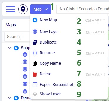
These options from the Map menu are also available in the context menu that comes up when right-clicking on a map or layer in the Maps list.

Global Scenario Filter

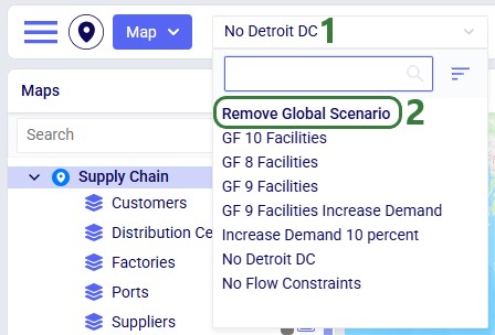
The Map Filters panel can be used to set scenarios for each map individually. If users want to use the same scenario for all maps present in the model, they can use the Global Scenario Filter located in the toolbar at the top of the Maps module:

1. The Global Scenario Filter will contain the text "Select Global Scenario" if no scenario has been selected. Click on the chevron icon on the right to open the drop-down list.
2. Users can use the free type text search box to quickly find the desired scenario in the drop-down list. Scenarios which contain the search text will be shown in the drop-down list.
3. The scenarios drop-down list can be sorted in 2 ways when clicking on this icon:
   
   1. Default: the scenarios are listed in the order they were added.
   2. A-Z Name: this sorts the scenario list in alphabetical order of scenarios names. Clicking on the A-Z Name sort order icon again will sort them in reverse alphabetical order.
4. The list of scenarios present in the model, select the desired one for all maps to use.

Now all maps in the model will use the selected scenario, and the option to set the scenario at the map-level is disabled.

When a global scenario has been set, it can be removed using the Global Scenario Filter again:

1. The "No Detroit DC" scenario has been selected as the global scenario to be used by all maps.
2. At the top of the scenarios list, there is now the option available to "Remove Global Scenario". Select this option to set the scenario by map instead of at the global level.

Persistence of Map Settings

The zoom level, how the map is centered, and the configuration of maps and their layers persist. After moving between other modules within Cosmic Frog or switching between models, when user comes back to the map(s) in a specific model, the map settings are the same as when last configured.

Adding and Configuring a Map

Now let us look at how users can add new maps, and the map configuration options available to them.

1. User has collapsed all pre-configured maps and chosen “New Map” from the Map drop-down menu. User can now type the name the new map should have into the text box. They have decided to call the new map “My New Map”.
2. On the right-hand side of the map, the New Map panel has come up, and user could have also typed the name here in the Map Name textbox.

Map Filters

Once done typing the name of the new map, the panel on the right-hand side of the map changes to the Map Filters panel which can be used to select the scenario and products the map will be showing. If the user wants to see a side-by-side map comparison of 2 scenarios in the model, this can be configured here too:

1. The Map Filters is the first of 3 panels users can use to configure maps. They can be selected by clicking on the 3 icons on the right. The first one is for Map Filters, the second one for Map Information, and the third one for Map Legend. Whichever one is active is colored darker blue than the other 2 icons. We will cover the Map Information and Map Legend panes with screenshots further below.
2. If there are multiple scenarios present in the model, user can select the one to show on the map from the drop-down list. Since this is a map-level setting it applies to all layers that are added to the map, and user can change between scenarios in this one place.
3. User can also choose to show the map for all products present in the model (the default) or a subset of them. When wanting to show a subset, user can click on the drop-down and select the product(s) to show:
   
   1. A search box to quickly filter the products list to those that contain certain text in their names is available to quickly find products of interest in case there are many products in the model.
   2. User also has the option to sort the product names either in the Default order, which is the order in which they were added to and appear in the Products table, or in (reverse) alphabetical order (the A-Z Name option).
   3. The checkbox(es) of the product(s) that should be shown on the map can be checked individually.

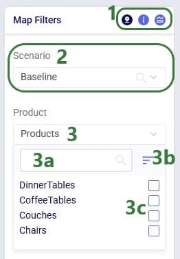
In the screenshot above, the Comparison toggle is hidden by the Product drop-down. In the next screenshot it is shown. By default, this toggle is off; when sliding it right to be on, we can configure which scenario we want to compare the previously selected scenario to:

1. The Comparison toggle has been turned on. A new empty map appears on the right-hand side of the map that is already showing the Baseline scenario.
2. In the Scenario drop-down, the user chooses the “No Detroit DC” scenario as the scenario to compare to the Baseline scenario.
3. If desired, the user can filter this second map for a subset of the Products available in the model using the Product drop-down list. Note that in order to have an apples-to-apples comparison between the 2 selected scenarios, the user should select the same product(s) for both scenarios using the 2 Product filters.
4. In the Map Legend of each map, we see that the left map now shows the Baseline scenario and the right map the No Detroit DC scenario. On the map itself, we see that the customers served by the DC in Detroit in the Baseline scenario are now served by the Chicago, Philadelphia and Atlanta DC’s in the No Detroit DC scenario.
5. Users can adjust both maps (e.g. panning, zooming, maximizing/minimizing) using either map. A change made to map on the left, will also be made to the map on the right, and vice versa.
6. The Apply to All toggle can be used to apply the same comparison filter settings for all maps within the model. By default, it is turned off: slide it to the right to turn it on. It will then be applied to any map that is already open or any map that will be opened while the toggle is on.

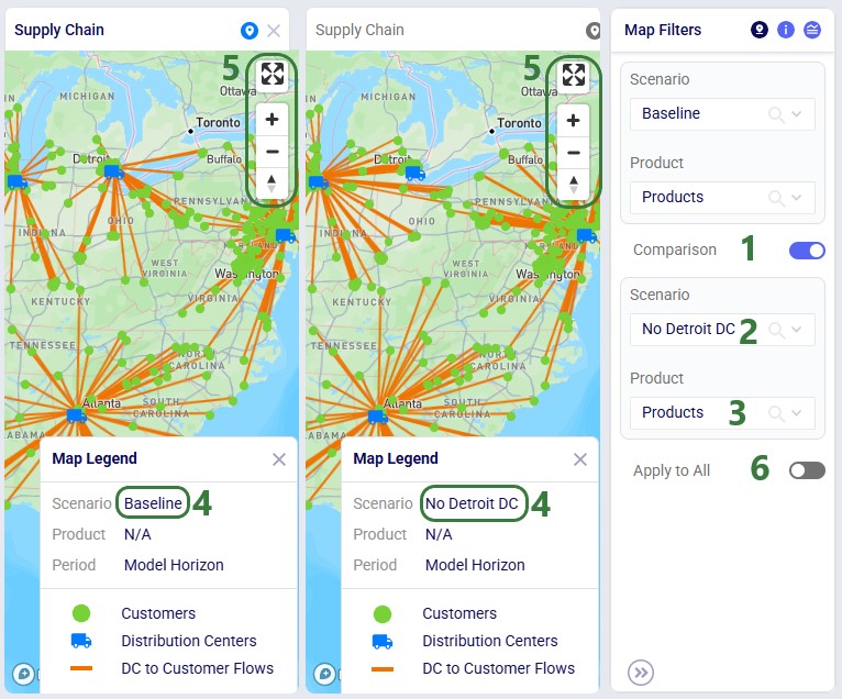
Please note:

• Combining the Global Scenario Filter with the Apply to All toggle for map comparisons, lets users configure comparisons between the same 2 scenarios for all maps in their model in 2 easy steps.  
• The Apply to All toggle for scenario comparisons appears in the Map Filters panel of each map. If it is turned on in any of the maps, it will be shown as on for all maps.
  
  • While the Apply to All toggle is on then if the scenario and/or product filters in the Comparison section are changed in any of the open maps, they are changed for all maps.
  • If the Apply to All toggle is turned off in any of the maps, either the one it was first turned on for or in any other map, it will be turned off for all maps. The comparisons in all open maps are reverted to the settings they had when the toggle was first turned on.

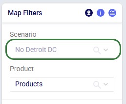
Instead of setting which scenario to use for each map individually on the Map Filters panel, users can instead choose to set a global scenario for all maps to use, as discussed above in the Global Scenario Filter section. If a global scenario is set, the Scenario drop-down on the Map Filters panel will be disabled and the user cannot open it:

Map Information

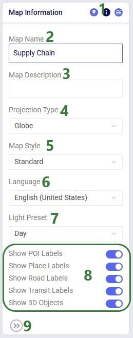
On the Map Information panel, users have a lot of options to configure what the map looks like and what entities (outside of the supply chain ones configured in the layers) are shown on it:

1. The second icon has been clicked to show the Map Information panel.
2. The Map Name is shown here and can be changed if desired.
3. A description of the map can be typed here. This is for example useful for a user when coming back to a map at a later stage to quickly be reminded of how and why the map is set up the way it is and for models shared between multiple users.
4. Projection Type: a map projection is a way to flatten the earth’s surface onto a screen. There are different methods to project the earth, and multiple options are available for Cosmic Frog maps. An explanation of the available projections together with some advantages and disadvantages of each can be found in this Map Projections documentation from Mapbox.
5. Map Style: multiple map styles are available to the user to choose from to show the map. The styles available are listed in the Mapbox Styles documentation from Mapbox, where user can see an example of each style.
6. Language: many languages are available to choose from in the drop-down list. The written names of features shown on the map are then displayed in the chosen language when available.
7. When the Standard Map Style is used (bullet 5), a Light Preset drop-down is available with 4 available options: Dusk, Dawn, Day, and Night. This will then show the map with the lighting as expected during that time of day/night.
8. Depending on the Map Style (bullet 5), some or all of the following features can be turned on or off on the map. Note that to see some of these labels, users may need to zoom in quite far:
   
   1. POI Labels: when turned on shows points of interests like restaurants, hotels, etc.
   2. Place Labels: when turned on shows names of countries, provinces/states, cities, etc.
   3. Road Labels: when turned on shows road names and numbers.
   4. Show Transit Labels: when turned on shows airport codes, names of sea routes, ports, etc.
   5. Show 3D Objects: when turned on objects like buildings will be shown with 3 dimensions while in the street view mode shown in the screenshot in the Keyboard & Mouse Actions on Maps section further above.
9. Click on this icon with 2 greater than signs to hide the Map Information pane. The icon then turns into 2 less than signs, which when clicked on will open the Map Information pane up again.

Map Legend

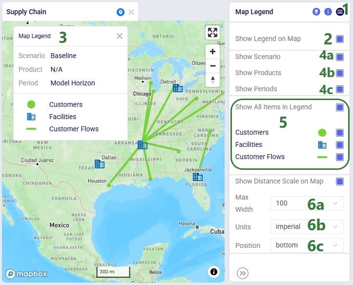
Users can choose to show a legend on the map and configure it on the Map Legend pane:

1. The third icon has been clicked to show the Map Legend panel.
2. Enabling this “Show Legend on Map” checkbox will put a legend on the map. If this checkbox is disabled, the map is shown without the legend.
3. This is the legend showing on the map. Note that users can click on the legend and drag it to a different location on the map. Hovering over Scenario, Product, or Period will also show the full text in a tooltip, which is helpful in case the text is too wide for it to be shown in the legend entirely.
4. In this section user can choose which of the following map settings should be included in the legend:
   
   1. Scenario – show in the legend for which scenario each layer is being drawn on the map.
   2. Product – show in the legend for which product(s) each layer is being drawn on the map. Will say “N/A” in case all products are being shown.
   3. Period – show in the legend for which period each layer is being drawn on the map. Will say “Model Horizon” for single-period models.
5. In this section user can choose which of the layers present in the map should be shown in the legend. Note that only layers that are currently enabled are listed here. Enabling the “Show All Items in Legend” checkbox will ensure all layers that are showing on the map (e.g. enabled in the Maps list) will be listed in the legend, this will automatically update the legend when user enables/disables layers in the Maps list. Disabling this checkbox will disable the checkboxes of all layers listed beneath it and no layers will be listed in the legend.
6. User can choose to show the distance scale on the map. If showing, following can be configured for the scale:
   
   1. Max Width – how wide the scale drawn on the map can be at the most. This number represents the number of pixels.
   2. Units – the unit of measure used for the scale. Options are imperial (distance in miles), metric (distance in kilometres), and nautical (distance in nautical miles).
   3. Position – the location on the map where the scale should be showing. Options are: top-left, top, top-right, right, bottom-right, bottom, bottom-left, and left.

Adding and Configuring Layers

To start visualizing the supply chain that is being modelled on a map, user needs to add at least 1 layer to a map, which can be done by choosing “New Layer” from the Map-menu:

1. User can now type the name the new layer should have into the text box. They have decided to call the new layer “My new Layer”.
2. On the right-hand side of the map, the Add Layer panel has come up, and user could have also typed the name here in the Layer Name textbox.

Condition Builder

Once a layer has been added or is selected in the Maps list, the panel on the right-hand side of the map changes to the Condition Builder panel which can be used to select the input or output table and any filters on it to be used to draw the layer:

1. The Condition Builder is the first of 3 panels users can use to configure map layers. They can be selected by clicking on the 3 icons on the right. The first one is for Condition Builder, the second one for Layer Style, and the third one for Layer Labels. Whichever one is active is colored darker blue than the other 2 icons.
2. The name of the layer is shown at the top of this panel. It cannot be changed here; should a user want to change the name of a layer, the “Rename” option in the Maps-menu can be used (also accessible from the right-click context menu when clicking on the layer in the Maps list).
3. The table to be used to draw the map layer can be chosen from the Table Name drop-down list. When clicking on the drop-down (caret down icon), a search box in which user can type text to find tables containing that text in their name becomes available. User can also sort the tables, either in the Default order (input tables first, then output tables, both in the order they appear in Cosmic Frog when sorting them by the Default in the Data module) or in (reverse) alphabetical order when choosing the A-Z Name sort order option.
   
   1. Three input tables are available in this list: Customers, Facilities, and Suppliers, which will draw these locations on the map (if geocoded). In addition to these 3 input tables, many output tables for the different engines are available too. An additional transportation optimization (Hopper) specific table called “TransportationRoutesMapLayer” is also available. This is not an input or output table, but one available specifically for the purpose of drawing multi-stop routes on the map. Here, the OptimizationFlowSummary output table is selected.
4. If all data in the selected table should be used to draw the map layer, then the user does not need to do anything in addition and the layer will be drawn according to the map-level scenario and product filters (see above section on Map Filters). If the table should be filtered before drawing the map layer, users have 2 options: either use Named Filters or the Condition Builder. The latter has been selected here; Named Filters will be covered further below.
5. When “Condition Builder” is chosen as the method to filter the table, then the user needs to specify the filter that will be applied in the Condition text box. Here, the user has typed flowtype = ‘CustomerFulfillment’, this means that only those records from the OptimizationFlowSummary table where the FlowType field value equals CustomerFulfillment will be drawn. To learn more about the syntax for writing conditions, please see this Help Center article.
6. The Record Count indicates the number of records that are used to draw the layer; this number will automatically update based on the condition(s) applied to the layer. As we will see in the next screenshot, this number does not necessarily match the number of lines/points shown on the map for this layer. Here 3,999 records will be used.
7. Users have the option to view a grid preview to ensure the correct filtered records are being used to draw the layer on the map. When toggled on, the preview will be shown in the central part of Cosmic Frog instead of the map itself.
8. Users have the option to display detailed waypoint routes on the road network instead of straight lines. This feature is available for the TransportationRoutesMapLayer and OptimizationFlowSummaryRoutes tables; see the Waypoint Routes help center article for more details.
9. Click on this icon with 2 greater than signs to hide the Condition Builder pane. The icon then turns into 2 less than signs, which when clicked on will open the Condition Builder pane up again.

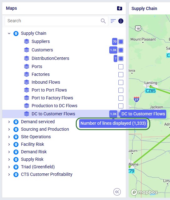
When looking at the DC to Customer Flows layer in the Maps list, we see that the Number of lines displayed in it is 1,333:

The condition used in the Condition Builder (flowtype = 'CustomerFulfillment') filters out 3,999 records in the OptimizationFlowSummary output table for the Baseline scenario. However, since each customer receives 3 different products (all from the same DC), the number of source destination pairs, and therefore the number of lines on the map, is 1,333.

We will now also look at using the Named Filters option to filter the table used to draw the map layer:

1. We are still looking at he DC to Customer Flows layers, same as above.
2. In the Condition Builder pane of this layer, user has chosen to use Named Filters. See also the “Named Filters in Cosmic Frog” Help Center article to learn all the ins and outs of Named Filters.
3. When clicking on the Named Filters drop-down, following become available to the user:
   
   1. A search box to quickly filter the named filter list to those that contain certain text in their names to quickly find filters of interest.
   2. Users also have the option to sort the named filters either in the Default order, which is the order in which they were added in the table, or in (reverse) alphabetical order (the A-Z Name option).
   3. The checkbox of the named filter that should be used to draw the layer on the map can be checked.

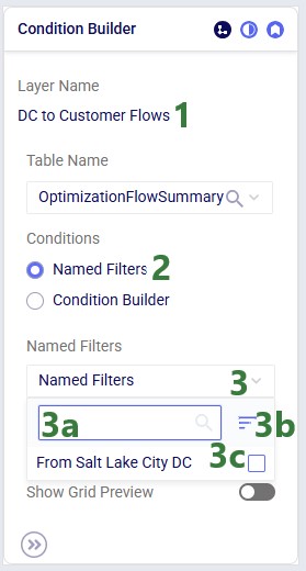
In this walk-through example, user chooses to enable the “From Salt Lake City DC” named filter:

1. The “From Salt Lake City DC” named filter has been enabled and is now shown beneath the Named Filters drop-down list. To remove this filter, the user can click on the x-icon on the right. If the whole name is not visible, the user can hover over the name of the filter to show the tooltip, which will show the full name of the named filter.
2. We see that the number representing the number of records used to draw the map layer has now correctly changed to 273.
3. The Show Grid Preview option is available here too, and the user has turned this on by sliding the toggle to the right.
4. The Filter Grid Preview is now shown in the central part of Cosmic Frog instead of the map itself.
5. The name of the Named Filter is showing at the right top of the Grid Preview. It can be removed by clicking on the x-icon on the right. Again, users can hover over the name to see the full name of the named filter in case it is truncated.
6. The record count of the records matching the Named Filter is repeated here too.
7. We can see in the preview that only records where the OriginName value is "Salt Lake City DC" are included.

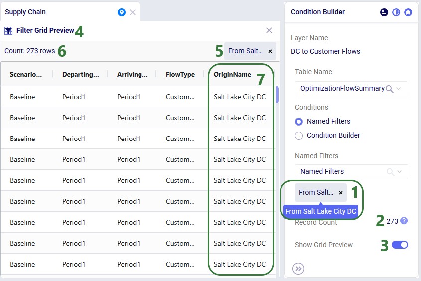
Similar to above, these 273 filtered records result in fewer lines (91) drawn on the map, since each customer served by the Salt Lake City DC receives 3 products from it. Therefore, the number of unique origin-destination pairs is 273 / 3 = 91.

Layer Style

In the next layer configuration panel, Layer Style, users can choose what the supply chain entities that the layer shows will look like on the map. This panel looks somewhat different for layers that show locations (Type = Point) than for those that show flows (Type = Line). First, we will look at a point type layer (Customers):

1. The Layer Style is the second of 3 panels users can use to configure map layers. It is opened by clicking on the middle icon of the 3 on the right, which is then colored in a darker blue than the other 2.
2. The name of the layer is shown at the top of this panel. It cannot be changed here; should a user want to change the name of a layer, the “Rename” option in the Maps-menu can be used (also accessible from the right-click context menu when clicking on the layer in the Maps list).
3. The Type of layer is listed, since this layer shows locations (the customers), the type is a Point layer, which cannot be changed.
4. In the Shape drop-down, user can choose the icon to show for this entity on the map. Circle has been chosen here.
5. The color with which the entity will be drawn on the map can be chosen from the Color drop-down.
6. The size in pixels of the shape drawn on the map can be configured here by dragging the slider to the right to increase the size and to the left to decrease the size.
7. When collision detection is turned on by moving the toggle to the right (it will then become blue), it is automatically determined if entities overlap with each other, and if so, mitigating actions are taken to show them not overlapping on the map.
8. The opacity level determines if the entities drawn by the layer are entirely solid (100% opacity) and obscuring the rest of the map beneath the entity or if the entity is somewhat transparent and the features of the map beneath it can be made out to some extent. The opacity level can be configured by dragging the slider to the right to increase the opacity and to the left to decrease the opacity.

Next, we will look at a line type layer, Customer Flows:

1. The Layer Style is the second of 3 panels users can use to configure map layers. It is opened by clicking on the middle icon of the 3 on the right, which is then colored in a darker blue than the other 2.
2. The name of the layer is shown at the top of this panel. It cannot be changed here; should a user want to change the name of a layer, the “Rename” option in the Maps-menu can be used (also accessible from the right-click context menu when clicking on the layer in the Maps list).
3. The Type of layer is listed, since this layer shows flows (the Customer Flows), the type is by default set to Line, which will draw solid lines on the map. User can change this by choosing one of following options from the Type drop-down: Line, Dashed (Long Dashes), Dotted, or Dashed Dotted.
4. The color with which the lines will be drawn on the map can be chosen from the Color drop-down.
5. The thickness of the lines drawn on the map can be configured here by dragging the slider to the right to increase the thickness and to the left to decrease the thickness.
6. The opacity level determines if the entities drawn by the layer are entirely solid (100% opacity) and obscuring the rest of the map beneath the entity or if the entity is somewhat transparent and the features of the map beneath it can be made out to some extent. The opacity level can be configured by dragging the slider to the right to increase the opacity and to the left to decrease the opacity.
7. Lines can optionally have a border, which can be turned on by moving the toggle to the right (it then becomes blue). If a line border is being used, its color can be chosen in the Color drop-down.
8. Also optionally, arrows indicating the direction of the flow the lines represent can be drawn on the lines. This can be turned on by moving the toggle to the right (it then becomes blue). If Line Direction is turned on, user can choose the color of the arrowheads in the Color drop-down and how far apart the arrowheads need to be by dragging the Spacing slider left (closer together) or right (farther apart). The orange box with the number 8 on the map shows one of these arrowheads indicating the direction of the customer flow.

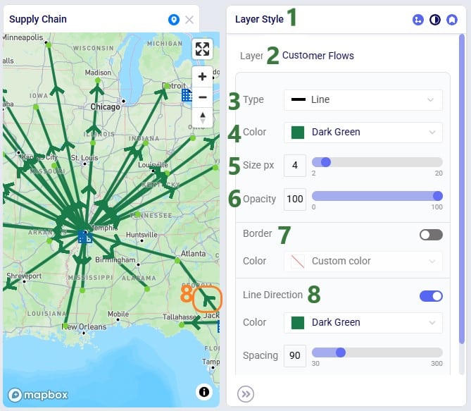
At the bottom of the Layer Style pane a Breakpoints toggle is available too (not shown in the screenshots above). To learn more about how these can be used and configured, please see the "Maps - Styling Points & Flows based on Breakpoints" Help Center article.

Layer Labels

Labels and tooltips can be added to each layer, so users can more easily see properties of the entities shown in the layer. The Layer Labels configuration panel allows users to choose what to show as labels and tooltips, and configure the style of the labels:

1. The third icon has been clicked to show the Layer Labels panel.
2. The name of the layer is shown at the top of this panel. It cannot be changed here; should a user want to change the name of a layer, the “Rename” option in the Maps-menu can be used (also accessible from the right-click context menu when clicking on the layer in the Maps list).
3. In the Labels drop-down list, the user can choose which field from the input/output table will be used as the label. Here the FlowQuantity field is chosen.
4. The font color of the label can be set in the Color drop-down list. Blue Black is the choice here.
5. The font size of the label can be set in the Size drop-down list. Size 14 is chosen here.
6. A background box for the label can be turned on (toggle to the right, color blue). If it is turned on, the color of it can be chosen from the drop-down list. Here the background is turned on and Pale Green is chosen as the background color.
7. Where the labels are shown on the map in relation to the entity they belong to can be chosen here from the Position drop-down list. Options are: Top, Bottom, Left, and Right.
8. In addition to a label that is always shown on the map, users can also enable tooltips which will show the value of 1 or multiple fields from the table the layer is drawn from when hovering over the entity on the map. The sser needs to enable the checkbox(es) of the field(s) of interest in the Tooltips list. These fields appear in the tooltip in the order they were checked in the Tooltips list.
9. The Display Aggregates toggle shows a SUM or AVG tag for numerical fields in the tooltip, based on how its aggregate is calculated. Users can choose to turn this off, for example once they feel comfortable they know what aggregate type is used for which field.

This next screenshot shows the tooltip of a flow line on the DC to Customer Flows layer. The tooltip is configured to show the following fields from the OptimizationFlowSummary table: OriginName, DesintationName, ProductName, FlowQuantity, TransportationCost, and TransportationTime. Display Aggregates is turned on:

1. These are the SUM and AVG tags shown for numerical fields to indicate the type of aggregate to calculate their tooltip values. Since this line represents the flow for 3 different products over the whole modeling horizon, the Flow Quantity is the sum of the flows of all products in all periods between this origin and destination.
2. For fields which can have multiple text values, the number of distinct values is shown with a blue background. Clicking on this ProductName field pins the tooltiptothemap and opens the Details to the right of the map with the ProductName expanded (see also next screenshot).
3. Clicking anywhere on this top area of the tooltip pins it to the map. The pin icon will then become darker blue. To unpin, click in this area again or anywhere else on the map.

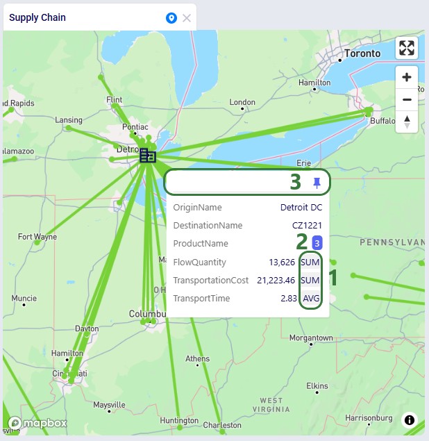
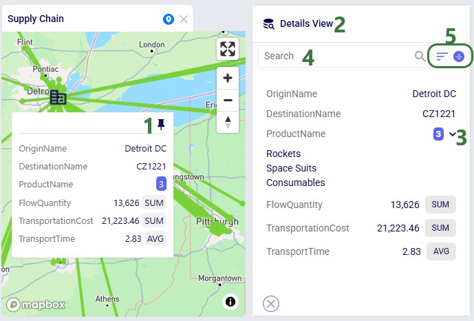
When pinning a tooltip, the Details View is shown on the right-hand side of the map:

1. The tooltip has been pinned to the map, the pin icon is now a darker shade of blue.
2. The Details View for this pinned tooltip has been opened.
3. For fields with multiple text values, the field can be expanded using the caret icon in order to review all value. By default these are collapsed, however, they will be expanded on opening if pinning the tooltip by clicking on the field with the multiple values in the tooltip (here by clicking on the ProductName field in the tooltip whilst it is not pinned).
4. Use the Search box to quickly search the field names and values of fields with multiple text values to filter them out.
5. Sort options (Default for the order as in the tooltip, A-Z for alphabetical, and clicking again for the reverse of these) and Collapse/Expand all options for the fields with multiple text values are available too.

Finally, this example shows a map where the labels for a customer locations layer are showing. They have been configured to use blue black as the font color, 14 as the font size, to use a background color which is set to cyan, and they are positioned below (position = bottom) the customer's map icon:

Maps of Multi-period Models

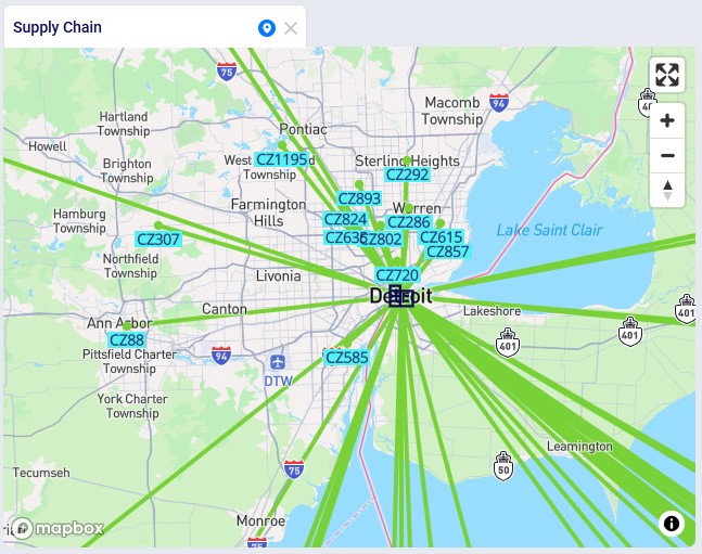
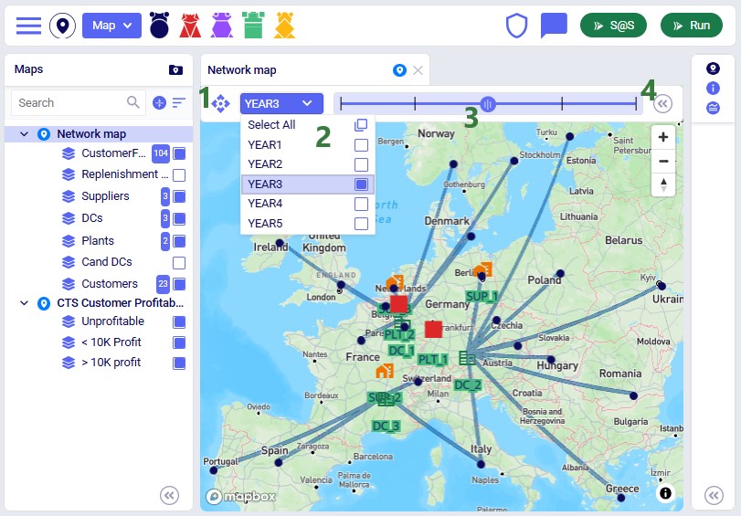
When modelling multiple periods in network optimization (Neo) models, users can see how these evolve over time using the map:

1. On the maps of multi-time period models, a toolbar controlling the periods shown on the map will be shown. This toolbar can be moved by clicking on the navigation icon on the left and dragging the toolbar to its desired location.
2. In the Period drop-down list, users can choose the period(s) for which they want to show the currently selected map. They also have the option to select multiple periods or all of them.
3. Instead of choosing a period from the drop-down mentioned in the previous bullet, users can also drag the dot on the timeline to the period they want to show the map for.
4. Use the icon with 2 less than signs to collapse the periods toolbar. When collapsed, clicking on the icon with 2 greater than icons will expand the periods toolbar again.

Adding a Location using the Map

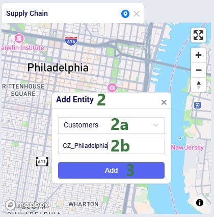
Users can now add Customers, Facilities and Suppliers via the map:

1. Zoom in and move the cursor to the location on the map where the Customer, Facility or Supplier should be added.
2. Right-click on the map and the Add Entity form comes up:
   
   1. From the drop-down list choose the table the location needs to be added to, either Customers, Facilities or Suppliers. Here a new Customer location is being added.
   2. Type the name of the new location, here the new customer will be called CZ_Philadelphia.
3. Click on the Add button to add the entity to the input table. In case user does not want to add the entity at this time, they can click on the x at the right top of the Add Entity form.

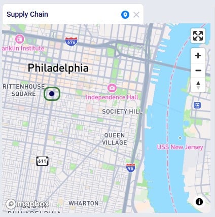
After adding the entity, we see it showing on the map, here as a dark blue circle, which is how the Customers layer is configured on this map:

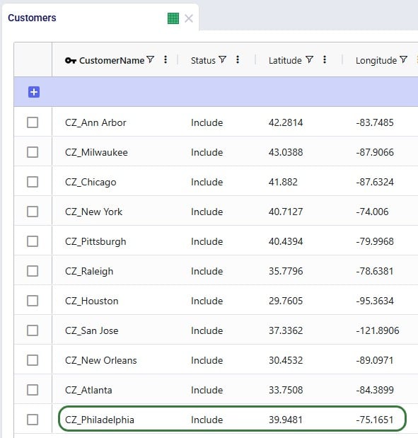
Looking in the Customers table, we notice that CZ_Philadelphia has been added. Note that while its latitude and longitude fields are set, other fields such as City, Country and Region are not automatically filled out for entities added via the map:

Example Maps

In this final section, we will show a few example maps to give users some ideas of what maps can look like. In this first screenshot, a map for a Transportation Optimization (Hopper engine) model, Transportation Optimization UserDefinedVariables available from Optilogic’s Resource Library (here), is shown:

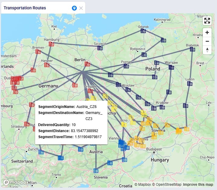
Some notable features of this map are:

• The customers have been color-coded based on the country they are in (e.g. red customers are in Germany, light blue in Austria, etc.). This is done by adding a layer for each country, choosing Customers as the table for each of these layers, filtering each for a different country using either the Condition Builder (Country = ‘Poland’, etc.) or Named Filters, and setting the color of the shape differently for each of these layers.
• The Transportation Routes Map Layer is used as the table to show the lines of the routes on the map.
  • The opacity of this Routes layer is set to 50%, so the features of the map are still somewhat visible through the lines.
• The Tooltip is configured on the Routes layer to show the value of 5 fields when hovering over a segment of the route:
  • Segment Origin Name
  • Segment Destination Name
  • Delivered Quantity
  • Segment Distance
  • Segment Travel Time

The next screenshot shows a map of a Greenfield (Triad engine) model:

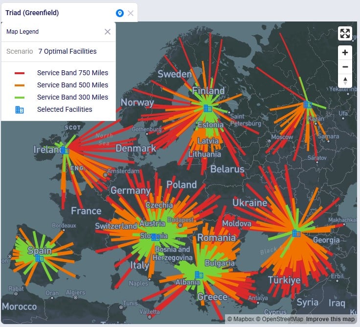
Some notable features of this map are:

• It shows the standard Triad (Greenfield) map for the “7 Optimal Facilities” scenario in the European Greenfield Facility Selection model, available from Optilogic’s Resource Library (here).
• The Projection Type is the default of Globe, but the Map Style has been changed to Navigation Night V1 (on the Map Information pane when selecting the map in the maps list).
• This model has 3 service bands set up in the Greenfield Service Bands input table: 50% of the demand quantity needs to be served from within 300 Miles, 70% from within 500 Miles, and 100% from within 750 Miles.
• Three layers that use the Optimization Greenfield Flow Summary output table as the table have been added, each filtered for 1 of the 3 service bands: servicebandname = ‘750 Miles’, etc., and each with a different color set up for the flow lines (green for 300 miles, orange for 500 miles, and red for 750 miles).

This following screenshot shows a subset of the customers in a Network Optimization (Neo engine) model, the Global Sourcing – Cost to Serve model available from Optilogic’s Resource Library (here). These customers are color-coded based on how profitable they are:

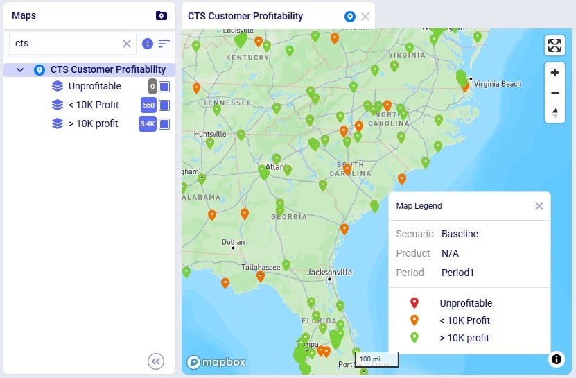
Some notable features of this map are:

• Three layers have been added, Unprofitable, <10k Profit, >10k Profit, all from the Optimization Cost To Serve Summary output table:
  • The condition used on the Unprofitable layer is as follows: (revenue - cost) < 0. The color used for the shapes of this layer is red, and since we do not see any red shapes on the map and there is a grey 0 as the record count for the layer, we can conclude there are no unprofitable customers in this scenario (Baseline) of this model.
  • The condition used on the <10k Profit layer is as follows: (revenue - cost) >= 0 and (revenue - cost) <= 10000. The color used for the shapes of this layer is orange. The record count for the layer indicates there are 568 such customers (not all shown in the screenshot), that are profitable, but with a profit less than $10k.
  • The condition used on the >10k Profit layer is as follows: (revenue - cost) > 10000. The color used for the shapes of this layer is green. The record count for the layer indicates there are 3.4k such customers (not all shown in the screenshot), that are profitable and have a profit greater than $10k.

Lastly, the following screenshot shows a map of the Tariffs example model, a network optimization (Neo engine) model available from Optilogic’s Resource Library (here), where suppliers located in Europe and China supply raw materials to the US and Mexico:

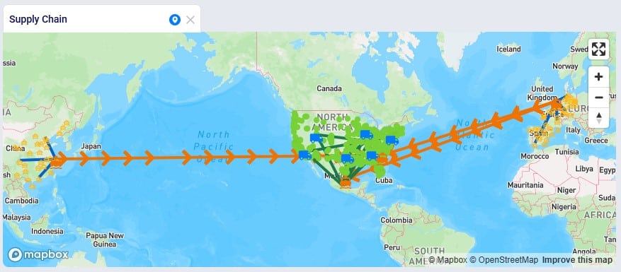
Some notable features of this map are:

• The Mercator projection is used, so the flows from China and Europe to the US and Mexico (the orange lines) can be shown in one view.
• The Line Direction option is used; the arrow heads on the orange lines indicate that the raw materials are coming from China/Europe and are being moved to Mexico/the US.
• Multiple layers that are using the Optimization Flow Summary output table as the table have been added so that the colors of the lines are indicative of the type of flow: blue lines for movements from suppliers to local ports (condition: FlowType = 'Procurement'), orange lines for movements between ports (condition: OriginName LIKE '%Port%' AND DestinationName LIKE '%Port%'), and green for movements from manufacturing locations to distribution centers (condition: OriginName LIKE '%Factory%').

We hope users feel empowered to create their own insightful maps. For any questions, please do not hesitate to contact Optilogic support at support@optilogic.com.

Cosmic Frog users can now visualize routes from Hopper (transportation optimization) and Neo (network optimization) on real road networks instead of straight lines. Valhalla, an open-source routing engine for OpenStreetMap, is used to calculate the waypoints.

This guide assumes familiarity with how to configure maps and their layers in Cosmic Frog. See the Getting Started with Maps help center article for the basics.

Quick Start

1. Add or select a map layer
2. Choose a table name:
   1. TransportationRouteMapLayer (Hopper), or
   2. OptimizationFlowSummaryRoutes (Neo)
3. Turn on the "Waypoint Routes" toggle
4. Click "Generate Routes"
5. Monitor progress in the Model Activity panel
6. View updated routes on the map

Why it Matters

• Realistic visualization: Understand how flows move along actual roads instead of straight lines
• Better analysis: Identify inefficiencies, and route overlap
• Improved communication: Stakeholders can better interpret results with familiar road-based visuals
• Scalable insights: Works across thousands of routes with clear progress tracking

How to Configure

There are 2 tables available in the Table Name drop-down on the Condition Builder panel of a map layer for which waypoint routes can be generated:

• TransportationRoutesMapLayer for Hopper - requires the TransportationSegmentSummary table to contain outputs for the scenario the map is currently showing
• OptimizationFlowSummaryRoutes for Neo - requires the OptimizationFlowSummary table to contain outputs for the scenario the map is currently showing

In both cases the configuration is similar; first we will cover a Hopper example and then a Neo example.

Hopper Walkthrough

1. The user has selected TransportationRoutesMapLayer as the table to use for the currently selected map layer (Routes - MK Artic); this layer shows routes which use the asset called "MK Artic".
2. The Waypoint Routes toggle can be turned on by the user if they want to generate detailed road network routes and display these on the map.

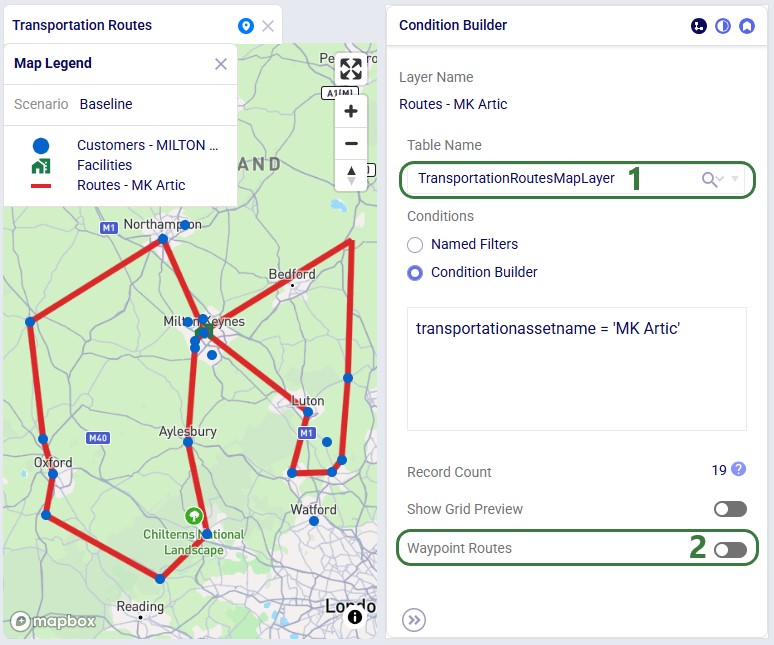
Please note:

• The Waypoint Routes toggle is disabled when an unsupported table is selected in the Table Name drop-down and the following warning is shown when hovering over the Waypoint Routes toggle:

• A warning is displayed in case the table needed to generate the waypoints is not populated:

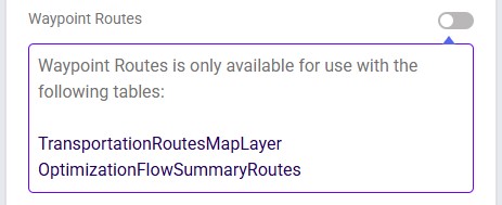
In our example case neither warning comes up, and the user turns on the Waypoint Routes option:

1. The user has switched the Waypoint Routes toggle to on.
2. The Skip Populated Routes toggle gives users the option to skip calculation of waypoints for routes that have already been calculated previously. The toggle is turned on by default to reduce calculation time. Turn this option off if coordinates have changed.
3. Click on the Generate Routes button to start the waypoint routes calculation.

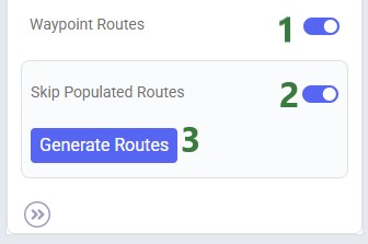
Processing time depends on the number of origin-destination pairs. As an indication, a larger Hopper model with ~3,000 routes took a little under 4 minutes to generate all waypoints.

Users can monitor the progress of the waypoint routes generation by opening the Model Activity panel:

1. To open the Model Activity panel, click on the blue speech bubble icon to the right in the toolbar across the top of Cosmic Frog.
2. We see that the routes calculation has already completed, indicated by the green check icon. A summary of how many routes were calculated successfully, how many failed, and how long it took is provided. Here, 19 routes were calculated in 2 seconds and none failed.

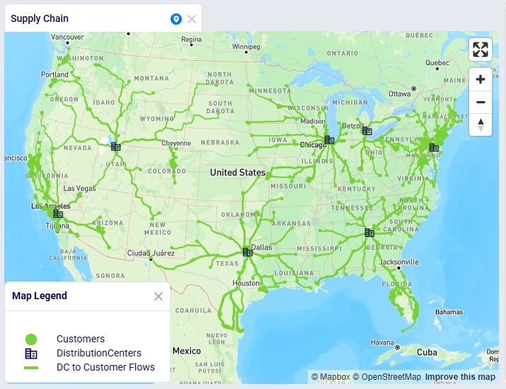
Once the calculation completes, the map is updated to show the routes the waypoints have been calculated for on the road network:

Neo Walkthrough

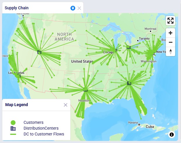
In this Neo example, we will generate road network flows for the following DC to Customer flows. This represents 1,333 unique origin-destination pairs:

1. Select the OptimizationFlowSummaryRoutes table from the Table Name drop-down.
2. Turn on the Waypoint Routes toggle.
3. Click on the Generate Routes button. While the waypoints are being calculated the button becomes greyed out and a spinner appears on it.
4. The user has opened the Model Activity panel, which shows:
   1. The routes that are currently being calculated. So far, it has calculated 880 of a total of 1,242 flows in about 3 minutes.
   2. The summary of routes that were calculated previously; 91 were calculated in about 14 seconds.

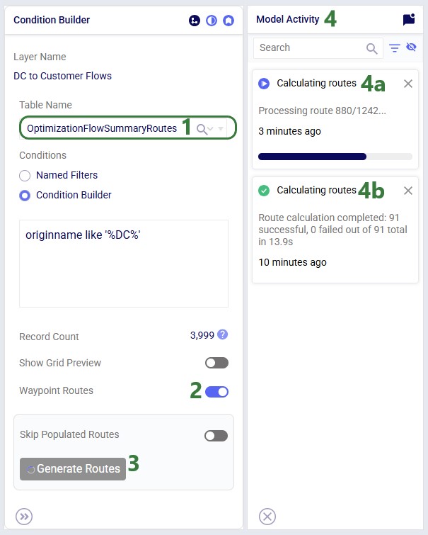
Once the waypoints have been calculated, the map updates and now looks as follows:

‍

‍

Other Helpful Resources

• Learn more about the Neo engine
• Learn the Hopper basics in this Getting Started article

Getting Started with Hopper

Hopper is the Transportation Optimization algorithm within Cosmic Frog. It designs optimal multi-stop routes to deliver/pickup a given set of shipments to/from customer locations at the lowest cost. Fleet sizing and balancing weekly demand can be achieved with Hopper too. Example business questions Hopper can answer are:

• What are the best routes and modes to minimize cost and maximize service?
• Is it better to ship on a route or ship direct via LTL or parcel?
• How can I optimize the mix of existing assets?
• What service improvements are possible based on different routing configurations?
• What is the best product mix per asset per route?
• What is the best carrier offer? What is best costing model to use?
• How can I best slot in new customers into existing routes? Or is it better to set up entirely new routes for new customers?
• How many transportation assets do I need to operate my routes?
• What is the most optimal stop sequence on my routes when combining deliveries and pickups (interleaved)?
• How do the interleaved routes change if I need to enforce Last In First Out (LIFO) rules?

Hopper’s transportation optimization capabilities can be used in combination with network design to test out what a new network design means in terms of the last-mile delivery configuration. For example, questions that can be looked at are:

• How is the proposed design going to change my current delivery design?
• What is my asset utilization going to be?
• Should I renegotiate any transportation agreements?
• Should my assets be located at their current domicile or is elsewhere better now?

With ever increasing transportation costs, getting the last-mile delivery part of your supply chain right can make a big impact on the overall supply chain costs!

It is recommended to watch this short Getting Started with Hopper video before diving into the details of this documentation. The video gives a nice, concise overview of the basic inputs, process, and outputs of a Hopper model.

In this documentation we will first cover some general Cosmic Frog functionality that is used extensively in Hopper, next we go through how to build a Hopper model which discusses required and optional inputs, how to run a Hopper model is explained, Hopper outputs in tables, on maps and analytics are covered as well, and finally references to a few additional Hopper resources are listed. Note that additional more advanced Hopper features are covered in separate articles:

• Network Transportation Optimization (Neo & Hopper)
• Multiple Compartments (Transportation Optimization)
• Territory Planning (Transportation Optimization)
• User-Defined Variables, Costs and Constraints (Transportation Optimization)‍

General Pointers before diving into Hopper Specifics

To not make this document too repetitive we will cover some general Cosmic Frog functionality here that applies to all Cosmic Frog technologies and is used extensively for Hopper too.

Using the Hopper Technology Filter

To only show tables and fields in them that can be used by the Hopper transportation optimization algorithm, disable all icons except the 4th (“Transportation”) in the Technologies Selector from the toolbar at the top in Cosmic Frog. This will hide any tables and fields that are not used by Hopper and therefore simplifies the user interface:

Information contained in Tooltips

Many Hopper related fields in the input and output tables will be discussed in this document. Keep in mind however that a lot of this information can also be found in the tooltips that are shown when you hover over the column name in a table, see following screenshot for an example. The column name, technology/technologies that use this field, a description of how this field is used by those algorithm(s), its default value, and whether it is part of the table’s primary key are listed in the tooltip.

UOM (unit of measure) Input Fields

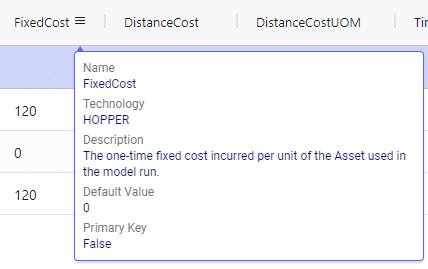
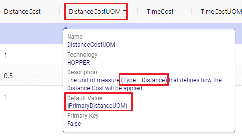
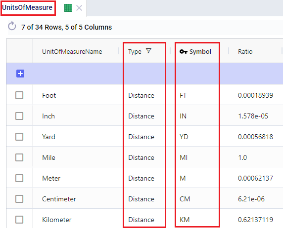
There are a lot of fields with names that end in “…UOM” throughout the input tables. How they work will be explained here so that individual UOM fields across the tables do not need to be explained further in this documentation as they all work similarly. These UOM fields are unit of measure fields and often appear to the immediate right of the field that they apply to, like for example Distance Cost and Distance Cost UOM in the screenshot above. In these UOM fields you can type the Symbol of a unit of measure that is of the required Type from the ones specified in the Units Of Measure table. For example, in the screenshot above, the unit of measure Type for the Distance Cost UOM field is Distance. Looking in the Units of Measure table, we see there are multiple of these specified, like for example Mile (Symbol = MI), Yard (Symbol = YD) and Kilometer (Symbol = KM), so we can use any of these in this UOM field. If we leave a UOM field blank, then the Primary UOM for that UOM Type specified in the Model Settings table will be used. For example, for the Distance Cost UOM field in the screenshot above the tooltip says Default Value = {Primary Distance UOM}. Looking this up in the Model Settings table shows us that this is set to MI (= mile) in our current model. Let’s illustrate this with the following screenshots of 1) the tooltip for the Distance Cost UOM field (located on the Transportation Assets table), 2) units of measure of Type = Distance in the Units Of Measure table and 3) checking what the Primary Distance UOM is set to in the Model Settings table, respectively:

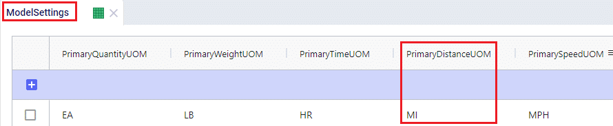
Note that only hours (Symbol = HR) is currently allowed as the Primary Time UOM in the Model Settings table. This means that if another Time UOM, like for example minutes (MIN) or days (DAY), is to be used, the individual UOM fields need to be used to set these. Leaving them blank would mean HR is used by default.

Status and Notes fields

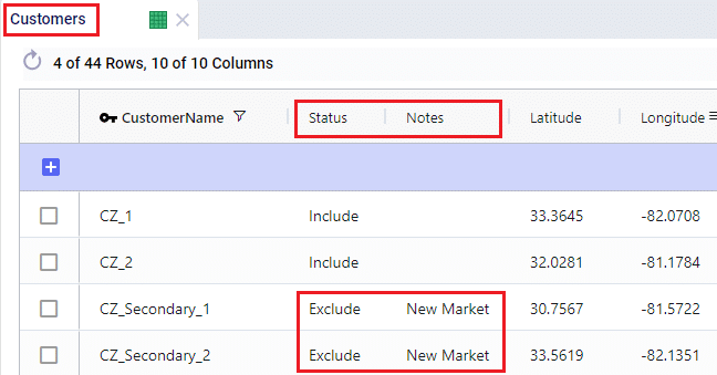
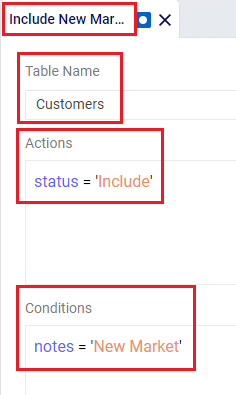
With few exceptions, all tables in Cosmic Frog contain both a Status field and a Notes field. These are often used extensively to add elements to a model that are not currently part of the supply chain (commonly referred to as the “Baseline”), but are to be included in scenarios in case they will definitely become part of the future supply chain or to see whether there are benefits to optionally include these going forward. In these cases, the Status in the input table is set to Exclude and the Notes field often contains a description along the lines of ‘New Market’, ‘New Product’, ‘Box truck for Scenarios 2-4’, ‘Depot for scenario 5’, ‘Include S6’, etc. When creating scenario items for setting up scenarios, the table can then be filtered for Notes = ‘New Market’ while setting Status = ‘Include’ for those filtered records. We will not call out these Status and Notes fields in each individual input table in the remainder of this document, but we definitely do encourage users to use these extensively as they make creating scenarios very easy. When exploring any Cosmic Frog models in the Resource Library, you will notice the extensive use of these fields too. The following 2 screenshots illustrate the use of the Status and Notes fields for scenario creation: 1) shows several customers on the Customers table where CZ_Secondary_1 and CZ_Secondary_2 are not currently customers that are being served but we want to explore what it takes to serve them in future. Their Status is set to Exclude and the Notes field contains ‘New Market’; 2) a scenario item called ‘Include New Market’ shows that the Status of Customers where Notes = ‘New Market’ is changed to ‘Include’.

The Status and Notes fields are also often used for the opposite where existing elements of the current supply chain are excluded in scenarios in cases where for example locations, products or assets are going to go offline in the future. To learn more about scenario creation, please see this short Scenarios Overview video, this Scenario Creation and Maps and Analytics training session video, this Creating Scenarios in Cosmic Frog help article, and this Writing Scenario Syntax help article.

How to Build a Hopper model

A subset of Cosmic Frog’s input tables needs to be populated in order to run Transportation Optimization, whereas several other tables can be used optionally based on the type of network that is being modelled, and the questions the model needs to answer. The required tables are indicated with a green check mark in the screenshot below, whereas the optional tables have an orange circle in front of them. The Units Of Measure and Model Settings tables are general Cosmic Frog tables, not only used by Hopper and will always be populated with default settings already; these can be added to and changed as needed.

We will first discuss the tables that are required to be populated to set up a basic Hopper model and then cover what can be achieved by also using the optional tables and fields. Note that the screenshots of all input and output tables mostly contain the fields in the order they appear in in the Cosmic Frog user interface, however on occasion the order of the fields was rearranged manually. So, if you do not see a specific field in the same location as in a screenshot, then please scroll through the table to find it.

Input Tables Required to run Hopper

Customers

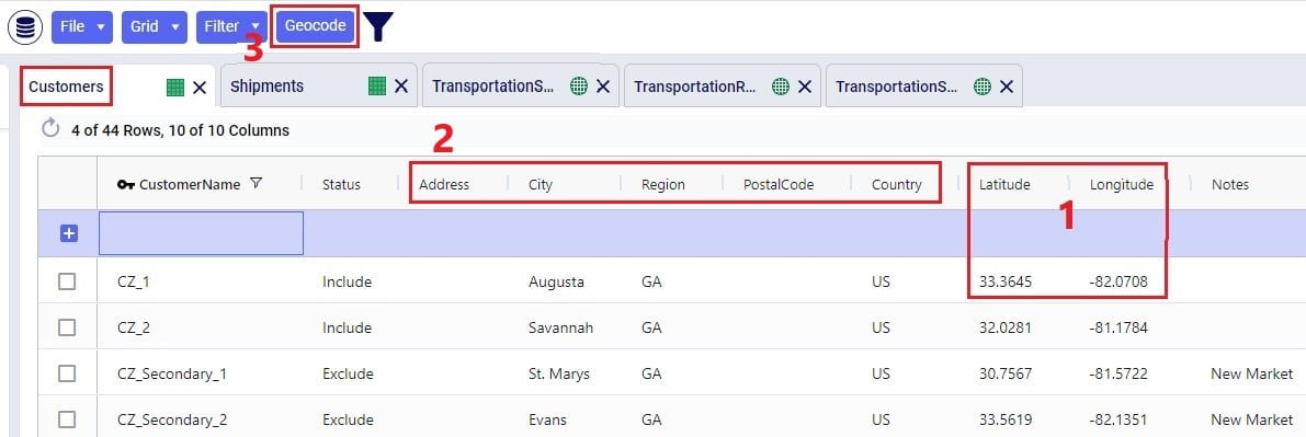
The Customers table contains what for purposes of modelling are considered the customers: the locations that we need to deliver a certain amount of certain product(s) to or pick a certain amount of product(s) up from. The customers need to have their latitudes and longitudes specified so that distances and transport times of route segments can be calculated, and routes can be visualized on a map. Alternatively, users can enter location information like address, city, state, postal code, country and use Cosmic Frog’s built in geocoding tool to populate the latitude and longitude fields. If the customer’s business hours are important to take into account in the Hopper run, its operating schedule can be specified here too, along with customer specific variable and fixed pickup & delivery times. Following screenshot shows an example of several populated records in the Customers table:

1. Latitudes and longitudes are required for distance and transport time calculations, and to visualize customers on a map.
2. If the latitude and longitude fields are not populated for customers, then filling out some of the columns with location information (Address, City, Country, Postal Code, Country) and using the geocoding tool can retrieve and populate latitudes and longitudes for you.
3. The geocoding tool – see this help article Geo Providers for Geocoding and Distance and Time Calculations, and this training session video How to Use Cosmic Frog Maps and Geocoding on how to use the geocoding tool.

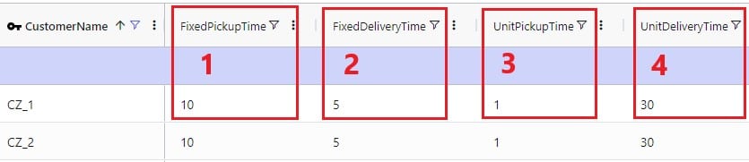
The pickup & delivery time input fields can be seen when scrolling right in the Customers table (the accompanying UOM fields are omitted in this screenshot):

1. Fixed Pickup Time – enter the amount of fixed time needed at this customer for pickups – applied once per pickup stop at this customer. Set to 10 minutes here (UOM field = MIN, not shown). It is additive to any Fixed Pickup Time specified on the Shipments and Transportation Assets tables.
2. Fixed Delivery Time – enter the amount of fixed time needed at this customer for deliveries – applied once per delivery stop at this customer. Set to 5 minutes here (UOM field = MIN, not shown). It is additive to any Fixed Delivery Time specified on the Shipments and Transportation Assets tables.
3. Unit Pickup Time – enter the amount of variable time needed at this customer for pickups – applied for each unit to be picked up at this customer. Set to 1 minute here (UOM fields set to MIN and EA, not shown). It is additive to any Unit Pickup Time specified on the Shipments and Transportation Assets tables.
4. Unit Delivery Time – enter the amount of variable time needed at this customer for deliveries – applied for each unit to be delivered at this customer. Set to 30 seconds here (UOM fields set to SEC and EA, not shown). It is additive to any Unit Delivery Time specified on the Shipments and Transportation Assets tables.

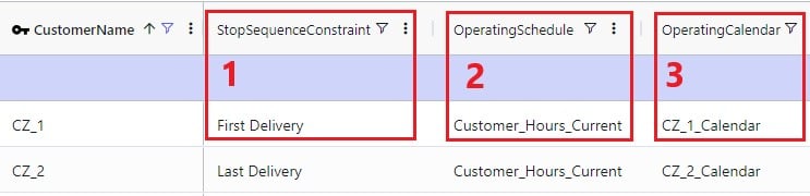
Finally, scrolling even more right, there are 3 additional Hopper-specific fields in the Customers table:

1. Stop Sequence Constraint – if the customer is required to be either the first or last stop on routes, this can be configured using this field. For customers to which deliveries are made, the available options are First Delivery or Last Delivery. For customers from which product is picked up, the options are First Pickup and Last Pickup.
2. Operating Schedule – the opening and closing times of locations for each day of the week can be entered into the Business Hours table which we will discuss as part of the optional Hopper input tables further below. Once these are set up, they can be used in this field on the Customers table to set the customer’s operating schedule; pickups & deliveries can then only be made during times that the customer is open. The name entered here needs to match one of the Schedule Names as specified on the Business Hours table. If no Operating Schedule is specified, the customer is assumed to always be open.
3. Operating Calendar – the dates during the modeling horizon that a location will be closed can be entered into Business Calendars table which we will discuss as part of the optional Hopper input tables further below. Once these are set up, they can be used in this field on the Customers table to set the customer’s operating calendar; pickups & deliveries can then only be made on dates that the customer is not closed. The name entered here needs to match one of the Calendar Names as specified on the Business Calendars table. If no Operating Calendar is specified, the customer is assumed to be open on all dates during the modeling horizon.

Facilities

The Facilities table needs to be populated with the location(s) the transportation routes start from and end at; they are the domicile locations for vehicles (assets). The table is otherwise identical to the customers table, where location information can again be used by the geocoding tool to populate the latitude and longitude fields if they are not yet specified. And like other tables, the Status and Notes field are often used to set up scenarios. This screenshot shows the Facilities table populated with 2 depots, 1 current one in Atlanta, GA, and 1 new one in Jacksonville, FL:

Scrolling further right in the Facilities table shows almost all the same fields as those to the right on the Customers table: Operating Schedule, Operating Calendar, and Fixed & Unit Pickup & Delivery Times plus their UOM fields. These all work the same as those on the Customers table, please refer to the descriptions of them in the previous section.

Products

The item(s) that are to be delivered to the customers from the facilities are entered into the Products table. It contains the Product Name, and again a Status and Notes fields for ease of scenario creation. Details around the Volume and Weight of the product are entered here too, which are further explained below this screenshot of the Products table where just one product “PRODUCT” has been specified:

1. The Unit Volume and Unit Volume UOM fields specify what the volume of 1 unit of the product is. Here this is 50 cubic feet (CFT). The Unit Volume is used to calculate the volume utilization of vehicles and ensure that on no segment of a route there is more volume on a vehicle than its capacity (in CFT) allows for. If volume is not important in your modelling, for example because your vehicles always weigh out before they cube out, then you could leave these fields blank and then it is assumed that the volume of 1 unit of product is equal to 1 using the primary volume unit of measure specified in the Model Settings table.
2. The Unit Weight and Unit Weight UOM fields specify what the weight of 1 unit of the product is. Here this is 265 pounds (LB). The Unit Weight is used to calculate the weight utilization of vehicles and ensure that on no segment of a route there is more weight on a vehicle than its capacity (in LB) allows for. If weight is not important in your modelling, for example because your vehicles always cube out before they weigh out, then you could leave these fields blank and then it is assumed that the weight of 1 unit of product is equal to 1 using the primary weight unit of measure specified in the Model Settings table.

Transportation Assets

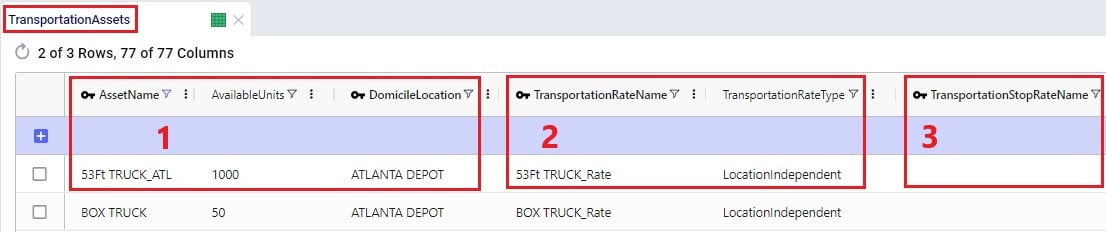
On the Transportation Assets table, the vehicles to be used in the Hopper baseline and any scenario runs are specified. There are a lot of fields around capacities, route and stop details, delivery & pickup times, and driver breaks that can be used on this table, but there is no requirement to use all of them. Use only those that are relevant to your network and the questions you are trying to answer with your model. We will discuss most of them through multiple screenshots. Note that the UOM fields have been omitted in these screenshots. Let’s start with this screenshot showing basic asset details like name, number of units, domicile locations, and rate information:

1. Specify the name of the vehicle in the Asset Name field, how many of the asset are available at this location in the Available Units field, and where it is based in the Domicile Location field. Notes:
   • If there is no limit on how many units of an asset can be available, then you can put a sufficiently large number in the Available Units field (like it has been done in this example, 1000 units) or leave it blank which will assume an infinite number of units are available.
   • If the Domicile Location is left blank, then it is assumed that this asset is available at all facilities. This field can use a group of Group Type = Facilities too.
2. Transportation Rate Name and Transportation Rate Type – many different types of costs that can be associated with a vehicle type can be set on the Transportation Rates table (discussed in the next section further below) and be applied to the vehicle by using the name of the transportation rate here in the Transportation Rate Name field. The Transportation Rate Type can be one of the following:
   • Location Independent – the cost structure does not depend on (the order of) the stops on the route.
   • Last Destination – Hopper will look up the correct cost structure based on the Route Destination Name of the Transportation Rate. Last Destination uses the customer visited last on the route.
   • Furthest Destination – Hopper will look up the correct cost structure based on the furthest customer from the origin Facility on the route.
3. Transportation Stop Rate Name – costs that are applied at the stops on the route can be specified in the Transportation Stop Rates table (discussed further below in the section on Hopper optional input tables) and be applied to an asset by using the name of the transportation stop rate here.

The following screenshot shows the fields where the operating schedule of the asset, any fixed costs, and capacity of the vehicles can be entered:

1. Operating Schedule – the start and end times of when assets are available each day of the week can be entered into the Business Hours table which we will discuss as part of the optional Hopper input tables further below. The name entered here needs to match a Schedule Name on the Business Hours table. If no Operating Schedule is specified, the vehicle is assumed to always be available.
2. Fixed Cost – a one-time fixed cost applied for each unit of the asset used in the model run.
3. Quantity Capacity – enter the capacity of the vehicle in terms of quantity. The Quantity Capacity UOM field specifies how this capacity is applied, e.g. per each or per dozen, etc.
4. Volume Capacity – enter the capacity of the vehicle in terms of volume. The Volume Capacity UOM field specifies how this capacity is applied, e.g. per cubic foot or per cubic meter, etc.
5. Weight Capacity – enter the capacity of the vehicle in terms of weight. The Weight Capacity UOM field specifies how this capacity is applied, e.g. per pound or per kilogram, etc.

Note that if all 3 of these capacities are specified, the most restrictive one will be used. If you for example know that a certain type of vehicle always cubes out, then you could just populate the Volume Capacity and Volume Capacity UOM fields and leave the other capacity fields blank.

‍

If you scroll further right, you will see the following fields that can be used to set limits on route distance and time when using this type of vehicle. Where applicable, you will notice their UOM fields too (omitted in the screenshot):

1. Max Distance To First Pickup – populate this field if there is an upper limit to how far this type of vehicle is allowed to travel empty (say from a depot) to its first pickup location (say a DC).
2. Max Distance Per Route – populate this field if there is an upper limit to how far this type of vehicle can travel on any one route.
3. Max Distance Between Stops – populate this field if there is an upper limit to how far this type of vehicle can travel between any 2 stops on a route.
4. Max Time Per Route – populate this field if there is an upper limit to how long this type of vehicle can travel on any one route.
5. Max Wait Time Per Route – when business hours are used at pickup and/or delivery locations, it is possible that an optimal route will need to have some wait time built into it. Use this field to limit the total time a vehicle type is allowed to wait during a route.

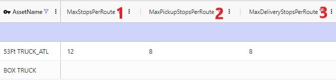
Limits on the amount of stops per route can be set too:

1. Max Stops Per Route – populate this field if there is an upper limit to the number of stops this type of vehicle can make on any one route, this field does not distinguish between stops where pickups are made or stops where deliveries are made.
2. Max Pickup Stops Per Route – populate this field if there is an upper limit to the number of stops where product is picked up from on any one route while using this vehicle.
3. Max Delivery Stops Per Route – populate this field if there is an upper limit to the number of stops where product is delivered to on any one route while using this vehicle.

A tour is defined as all the routes a specific unit of a vehicle is used on during the model horizon. Limits around routes, time, and distance for tours can be added if required:

1. Max Routes Per Tour – the maximum number of routes a vehicle can be used on during the model horizon.
2. Min Routes Per Tour – the lower limit on the number of routes a vehicle has to be used on during the model horizon.
3. Max Time Per Tour – the maximum amount of time a vehicle can be used over the model horizon. This is defined as from the start of its first route to the end of its last route.
4. Max Distance Per Tour – the upper limit on the distance a vehicle can travel together on all its routes during the model horizon.
5. Speed – populate this field if the speed of this type of vehicle is different from the Average Speed set in the Model Settings table.

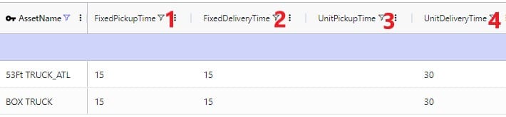
Scrolling still further right you will see the following fields that can be used to add details around how long pickup and delivery take when using this type of vehicle. These all have their own UOM fields too (omitted in the screenshot):

1. Fixed Pickup Time – enter the amount of fixed time that this type of vehicle needs at each pickup location. It is additive to any Fixed Pickup Time specified on the Shipments, Customers, and Facilities tables.
2. Fixed Delivery Time – enter the amount of fixed time that this type of vehicle needs at each delivery location. It is additive to any Fixed Delivery Time specified on the Shipments, Customers, and Facilities tables.
3. Unit Pickup Time – enter the amount of variable time that this type of vehicle needs at pickup locations for each unit. It is additive to any Unit Pickup Time specified on the Shipments, Customers, and Facilities tables.
4. Unit Delivery Time – enter the amount of variable time that this type of vehicle needs at delivery locations for each unit. It is additive to any Unit Delivery Time specified on the Shipments, Customers, and Facilities tables.

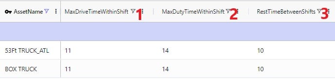
The next 2 screenshots shows the fields on the Transportation Assets table where rules around driver duty, shift, and break times can be entered. Note that these fields each have a UOM field that is not shown in the screenshot:

1. Max Drive Time Within Shift – the upper limit on how long a driver is allowed to drive the asset during a shift.
2. Max Duty Time Within Shift – the upper limit on how long a driver can work during a shift. This includes everything (driving, service time at a stop, wait time, short breaks, etc.) that is not a rest in between shifts, so effectively this field controls the length of a shift.
3. Rest Time Between Shifts – the minimum amount of rest time in between 2 shifts.

1. Max Drive Time Before Short Break – the upper limit on the cumulative time driving since the last rest or break after which a short break needs to be taken.
2. Short Break Time – the length of the break that needs to be taken once the max drive time before short break limit is reached.
3. Is Round Trip – when set to True, the vehicle will return to its domicile location at the end of a route; when set to False the route ends at the last stop.
4. Is Last In First Out – when set to True, shipments will be delivered in the reverse order of their pickups, modelling that a vehicle can only be loaded and unloaded from the back. This field will result in different interleaved and backhaul routes when set to True vs when set to False.

Limits around out of route distance can be set too. Plus details regarding the weight of the asset itself and the level of CO2 emissions:

1. Max Out Of Route Distance – this field and the next (Max Out Of Route Distance Percentage) can be used to set upper limits to the distance of a route as compared to the distance from the route origin location to the stop on the route that is farthest from the origin location. Consider the following route with 4 stops on it where stop 2 is farthest from the origin location:

1. • The out of route distance is defined as the distance of the multi-stop route (= the sum of the distances of the 4 green segments) minus twice the red distance from the origin to stop 2 (which is the stop farthest from the origin).
   • The distances used here for the multi-stop route and the distance to the farthest stop are those specified on the Transit Matrix table, if used, or otherwise based on the latitudes & longitudes of the locations plus the Circuity Factor specified in the Model Settings table.
2. Max Out Of Route Distance Percentage – instead of an absolute value for the Max Out of Route Distance allowed for a route that can be set using the previous field, this field can be used to set the upper limit of the out of route distance in terms of a percentage. If this field is set to 50 for example, the distance of the green multi-stop route can at a maximum be 50% more than 2 times the distance to the farthest stop on the multi-stop route. E.g. max route distance = 1.5 * 2 * red distance (distance to the farthest stop).
3. Asset Weight – the weight of 1 unit of the asset when empty; it is used for CO2 Emissions calculations.
4. CO2 Emission Rate – the rate of CO2 Emissions for this asset. These are applied based on the UOM field which can be Distance, Quantity-Distance, Volume-Distance or Weight-Distance
   • Distance: the CO2 Emission Rate is multiplied by the route’s total distance to calculate the CO2 Emissions of the route.
   • Quantity-Distance: the CO2 Emission Rate is multiplied by the total distance of the route and by the quantity delivered on the route to calculate the CO2 Emissions of the route.
   • Volume-Distance: the CO2 Emission Rate is multiplied by the total distance of the route and by the volume delivered on the route to calculate the CO2 Emissions of the route.
   • Weight-Distance: to calculate route’s CO2 emissions, the CO2 Emission Rate is multiplied by the total distance of the route and by the asset’s total weight, which includes the weight of the empty asset (see bullet 1 above) and the weight of the load delivered on the route.

Lastly, a default cost, fixed times for admin, and an operating calendar can be specified for a vehicle in the following fields on the transportation assets table:

1. Default Distance Cost – this distance based cost is used in cases where no transportation rate can be found for a route. If not provided, Hopper will treat any route with no transportation rate specified as invalid/infeasible.
2. Fixed Admin Time At Route Start – a certain set amount of time (say for paperwork) that is required to be spent at the start of each route.
3. Fixed Admin Time At Route End – a certain set amount of time (say for paperwork) that is require to be spent at the end of each route.
4. Operating Calendar – the dates during the modeling horizon that a vehicle cannot be used can be entered into Business Calendars table which we will discuss as part of the optional Hopper input tables further below. Once these are set up, they can be used in this field on the Transportation Assets table to set the asset’s operating calendar; pickups & deliveries can then only be made on dates that the vehicle is available for use. The name entered here needs to match one of the Calendar Names as specified on the Business Calendars table. If no Operating Calendar is specified, the asset is assumed to be available on all dates during the modeling horizon.

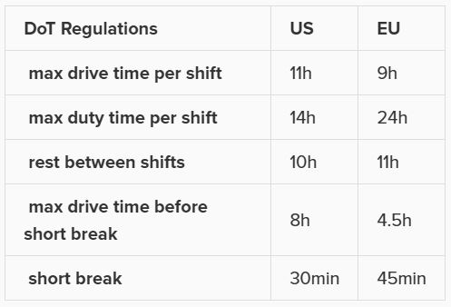
As a reference, these are the department of transportation driver regulations in the US and the EU. They have been somewhat simplified from these sources: US DoT Regulations and EU DoT Regulations:

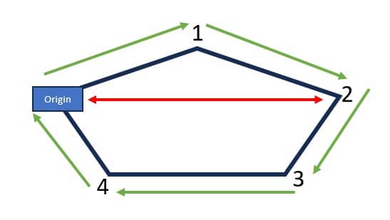
Consider this route that starts from the DC, then goes to CZ1 & CZ2, and then returns to the DC:

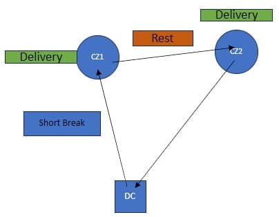
The activities on this route can be thought of as follows, where the start of the Rest is the end of Shift 1 and Shift 2 starts at the end of the Rest:

Notes on Driver Breaks:

• If service has commenced it will continue even if the duty clock is reached, a rest will be taken at the end of service.
• Short Breaks and Rests can be taken during Wait Time if there is enough time.
• A Short Break can trigger a Rest, in that case the Rest is taken right away and not a Short Break first.
• Breaks and Rests are currently based on individual routes as the assumption is that a driver starts each route with fresh clocks.

Transportation Rates

Except for asset fixed costs, which are set on the Transportation Assets table, and any Direct Costs which are set on the Shipments table, all costs that can be associated with a multi-stop route can be specified in the Transportation Rates table. The following screenshot shows how a transportation rate is set up with a name, a destination name and the first several cost fields. Note that UOM fields have been omitted in this screenshot, but that each cost field has its own UOM field to specify how the costs should be applied:

1. Transportation Rate Name – the name of the rate cost structure being specified in this record. This can be used in the Transportation Rate Name field on the Transportation Assets table to associate a cost structure with an asset.
2. Route Destination Name – the location name of the last or furthest delivery on the route when Rate Type is either Last Destination or Furthest Destination (set on the Transportation Assets table where the rate can be selected to be used). This dictates which record will be used to calculate the cost of that route. Notes:
   1. For Last/Furthest Destination Rate Types you will typically have multiple records in the Transportation Rates table that have the same Transportation Rate Name table which have different individual or grouped Route Destination Names to set up different costs for different Last / Furthest Destinations on the route.
   2. If a Rate Type of Location Independent is used in the Transportation Assets table, this field should be left blank.
3. Fixed Cost Per Route – a one time cost applied to each route using this rate structure.
4. Distance Cost – the cost that is applied per distance travelled on the route, this includes the segment where the asset is returned to its domicile location (the reposition segment of the route).
5. Reposition Distance Cost – the cost that is applied per distance when travelling while the asset is empty, for example on the segment of the route where the asset is returned to its domicile location (from the last stop on the route back to the origin location). This is in addition to any Distance Costs specified which will also be applied when travelling while empty.
6. Out Of Route Distance Cost – the cost that is applied per distance that is considered out of route, based on the definition of out of route distance given in the previous section on the Transportation Assets table. This is additive to any Distance and Reposition Distance Costs specified.

Scrolling further right in the Transportation Rates table we see the remaining cost fields:

1. Time Cost – the cost per unit of time that the asset is used.
2. Wait Time Cost – the cost per unit of time that the vehicle is waiting.
3. Rest Time Cost – the cost per unit of time during a rest in between 2 shifts.
4. Break Time Cost – the cost per unit of time that the driver is on a short break after the maximum drive time per shift is reached.
5. Stop Cost – the cost incurred by the asset at each stop.
6. Unit Cost – the cost per unit product that is delivered on the route. A single numeric value, a step cost, or a custom cost function can be used in this field. An example of using a Step Cost here is discussed in the section on the Step Costs table further below.

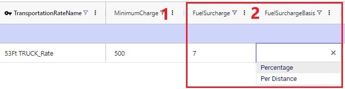
Finally, a minimum charge and fuel surcharge can be specified as part of a transportation rate too:

1. Minimum Charge – if the total costs on a route add up to less than the number specified here as the minimum charge, this minimum charge value will be used as the total route cost.
2. Fuel Surcharge and its Basis field – a surcharge which can be applied as a percentage or a per distance cost. When the basis is set to percentage, the fuel surcharge is calculated as Distance Cost * Fuel Surcharge/100. When the basis is set to Per Distance, the fuel surcharge is calculated as Route Distance * Fuel Surcharge.

Shipments

The amount of product that needs to be delivered from which source facility/supplier to which destination customer or picked up from which customer is specified on the Shipments table. Optionally, details around pickup and delivery times, direct costs, and fixed template routes can be set on this table too. Note that the Shipments table is Transportation Asset agnostic, meaning that the Hopper transportation optimization algorithm will choose the optimal one to use from the vehicles domiciled at the source location. This first screenshot of the Shipments table shows the basic shipment details:

1. ShipmentID – each Shipment needs to have its own unique identifier.
2. Source Name, Destination Name and Product Name – specify which Product needs to be delivered to which Customer from which Facility/Supplier or which product needs to be picked up from which Customer to be delivered to which Facility/Supplier. Each of these fields can also use Groups.
3. Quantity, Volume, and Weight (latter 2 not shown in screenshot), plus their UOM fields – the amount of product that needs to be delivered from this source to this destination, which can be specified in terms of quantity, volume, and/or weight.

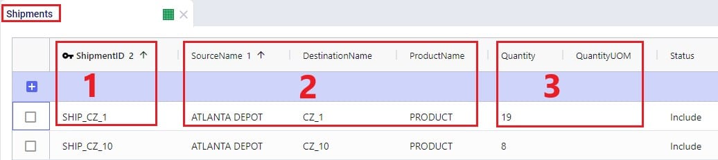
Here is an example of a subset of Shipments for a model that will route both pickups and deliveries:

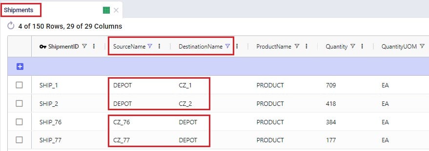
To the right in the Shipments table we find the fields where details around shipment windows can be entered:

1. Earliest Pickup Date – the date and time from when this shipment is allowed to be picked up from the source.
2. Latest Pickup Date – the date and time until when this shipment is allowed to be picked up from the source.
3. Earliest Delivery Date – the date and time from when this shipment is allowed to be delivered to the destination.
4. Latest Delivery Date – the date and time until when this shipment is allowed to be delivered to the destination.

Still further right on the Shipments table are the fields where details around pickup and delivery times can be specified:

1. Fixed Pickup Time – enter the amount of fixed time that this shipment needs at this pickup location. It is additive to any Fixed Pickup Time specified on the Transportation Assets table.
2. Fixed Delivery Time – enter the amount of fixed time that this shipment needs at this delivery location. It is additive to any Fixed Delivery Time specified on the Transportation Assets table.
3. Unit Pickup Time – enter the amount of variable time that this shipment needs at this pickup location for each unit. This Unit Pickup Time is additive to any Unit Pickup Time specified on the Transportation Assets table. Note that this Unit Pickup Time field on the Shipments table is more flexible than the one on the Transportation Assets table due to the use of the Unit UOM field which makes it possible to apply this variable time not only to Units of Measure of Type = Quantity but also to those of Type = Weight or Cubic. The Unit Pickup Time set on the Transportation Assets table uses a per each unit of measure which cannot be changed.
4. Unit Delivery Time – enter the amount of variable time that this shipment needs at this delivery location for each unit. This Delivery Time is additive to any Unit Delivery Time specified on the Transportation Assets table. Note that this Unit Delivery Time field on the Shipments table is more flexible than the one on the Transportation Assets table due to the use of the Unit UOM field which makes it possible to apply this variable time not only to Units of Measure of Type = Quantity but also to those of Type = Weight or Cubic. The Unit Delivery Time set on the Transportation Assets table uses a per each unit of measure which cannot be changed.

Finally, furthest right on the Shipments table are fields where Direct Costs, details around Template Routes and decompositions can be configured:

1. Direct Cost – if this field is populated with a number, then it is evaluated during the Hopper run if it is more beneficial (e.g. lower overall cost) to ship direct to this customer for the Direct Cost specified here than to put this customer on a multi-stop route. This can be used when considering LTL or Parcel options. Note that Cosmic Frog can connect to RateWare XL to retrieve LTL rates.
2. Template Route Name – if the user wants to fix certain routes, for example to how they are currently set up, then this field and the Template Route Stop Sequence field can be used. Here, specify the name of the route, which can be a number (like in this screenshot) or text, this Shipment needs to be on. Shipments with the same Template Route Name will be on the same route together. Leave this field blank if the Hopper algorithm should optimize the routes and determine which shipments should be on the same route and in which order.
3. Template Route Stop Sequence – this works with the Template Route Name field to fix routes to have specific shipments in a specific order on them. Here, specify the stop number for this Shipment on the Template Route, starting at 1 and increasing by 1 for each next stop. Leave this field blank if the Hopper algorithm should optimize the routes and determine which shipments should be on the same route and in which order.
4. Decomposition Name – shipments with the same Decomposition Name will be run together as a subproblem in the Hopper solve.

Note that there are multiple ways to switching between forcing Shipments and the order of stops onto a template route and letting Hopper optimize which shipments will be put on a route together and in which order. Two example approaches are:

1. Create 2 sets of Shipment records where one set has the Template Route Name and Template Route Stop Sequence fields populated to force specific routes and in the other set these fields are left blank so these Shipments can be optimized. Set the Status to Include of the set of Shipments that you want to be included by default and to Exclude of those that you do not want to be included by default. Use the Notes field for both sets, e.g. “forced routes” and “optimized routes” and use it to switch the Status from Include to Exclude for 1 set and Exclude to Include for the other set in scenarios.
2. Create 1 set of Shipment records that have the Template Route Name and Template Route Stop Sequence fields populated to force specific routes. Set the Status of these to Include and use the Notes field, for example put “original routes” in there. Then use the Notes field to filter out these fields in a scenario to set the Template Route Name and Template Route Stop Sequence fields to blank; the Shipments will then be optimized and not forced onto a template route in this scenario.

Optional Input Tables to use with Hopper

The tables and their input fields that can optionally be populated for their inputs to be used by Hopper will now be covered. Where applicable, it will also be mentioned how Hopper will behave when these are not populated.

Transit Matrix

In the Transit Matrix table, the transport distance and time for any source-destination-asset combination that could be considered as a segment of a route by Hopper can be specified. Note that the UOM fields in this table are omitted in following screenshot:

1. Origin Name, Destination Name, and Asset Name – specify the origin, destination, and transportation asset of the segment for which the transport distance and transport time are specified in this record. Each of these fields can also use Groups, however unless a modelling trick to achieve certain behavior/cost is used, this usually does not make sense to do for Origin Name and Destination Name as locations with different latitudes and longitudes will typically result in different distances. If Asset Name is left blank like in the screenshot above, the record applies to all vehicles that can be considered for this source-destination pair. Note that if you want to specify transport distances and/or transport times for all possible segments, this Matrix should contain records for:
   • Each Source Name and Destination Name of each Shipment (for the case where this Destination is the first stop on a Route) and the reverse (for the case where this Destination is the last stop on a Route).
   • Each Destination name to Each Destination name that have the same Source Name in the Shipments table, to consider all possible orders of stops on routes originating from this Source Name.
   • If transport distances and/or transport times are dependent on the vehicle travelling the segment, then repeat bullets a) and b) above for all Transportation Assets that can be used on the segment.
2. Transport Distance – set the distance for this segment and vehicle combination. It is for example possible that distances are dependent on vehicle type if certain vehicles cannot use certain roads while others can.
3. Transport Time – set the time it takes to travel from this source to this destination on specified vehicle.
4. Additional Cost – an additional cost that is incurred if this segment is used as part of a route. It is included in the Distance Cost in Hopper output tables.
5. IsSymmetric – if the transport distance and transport time are the same in both directions between the specified source and destination for the specified vehicle, then set this field to True (the default when left blank is also True). If set to True only 1 record for each source-destination-vehicle combination needs to be populated. If set to False, then 2 separate records for the source-destination-vehicle combination need to be populated where the source and destination are switched for the second record.

The transport distances for any source-destination pairs that are not specified in this table will be calculated based on the latitudes and longitudes of the source and destination and the Circuity Factor that is set in the Model Settings table. Transport times for these pairs will be calculated based on the transport distance and the vehicle’s Speed as set on the Transportation Assets table or, if Speed is not defined on the Transportation Assets table, the Average Speed in the Model Settings table.

Transportation Stop Rates

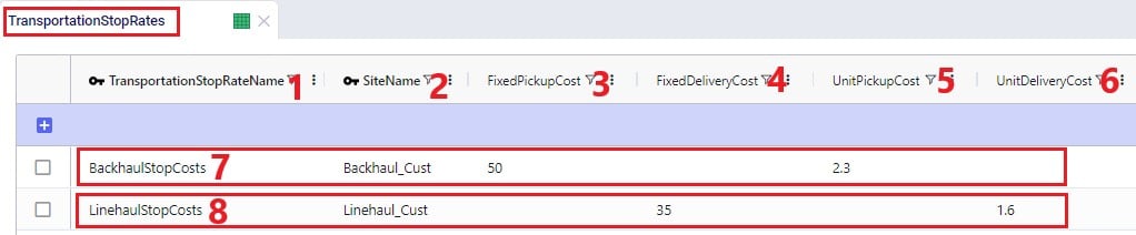
Costs that need to be applied on a stop basis can be specified in the Transportation Stop Rates table:

1. Transportation Stop Rate Name – the name of the rate being specified, which can be used in the Transportation Stop Rate Name field on the Transportation Assets table to associate these stop costs with a vehicle. Multiple records with the same Transportation Stop Rate Name together make up a rate.
2. Site Name – the stop(s) where this rate will be applied. It is possible to use a Named Filter saved on for example the Customers table or a Group name in this field to apply the stop rate to multiple locations.
3. Fixed Pickup Cost – a one time set cost applied when picking up at this stop.
4. Fixed Delivery Cost – a one time set cost applied when delivering to this stop.
5. Unit Pickup Cost – a variable cost applied per unit when picking up at this stop.
6. Unit Delivery Cost – a variable cost applied per unit when delivering to this stop.
7. A Stop Rate called BackhaulStopCosts is specified in this record. The Site Name is the named filter Backhaul_Cust that is set up on the customers table where the customer has “Backhaul” in the Notes field to indicate customers from which shipments will be picked up. For each pickup, there is a fixed cost of $50 that will be applied at each of these pickup stops and a variable cost of $2.30 per unit that is applied in addition.
8. A Stop Rate called LinehaulStopCosts is specified in this record. The Site Name is the named filter Linehaul_Cust that is set up on the customers table where the customer has “Linehaul” in the notes field to indicate customers to shipments will be delivered. For each delivery, there is a fixed cost of $35 that will be applied at each of these delivery stops and a variable cost of $1.60 per unit that is applied in addition.

Template Routes

If Template Routes are specified on the Shipments table by using the Template Route Name and Template Route Stop Sequence fields, then the Template Routes table can be used to specify if and how insertions of other Shipments can be made into these template routes:

1. Template Route Name and Asset Name – specifies which template route as entered on the Shipments table and vehicle (asset) combination this template route record applies to. Notes:
   • Template Route Name needs to match a Template Route Name used on the Shipments table for this record to be used.
   • If Asset Name is left blank it means that Hopper will pick the cheapest asset available to operate this template route.
2. Additional Shipment Insertion Type – this field specifies for the template route – asset combination if insertions of other shipments onto this route are allowed and if so how:
   • No Insertion – no additional Shipments can be inserted into this template route. This is the default if the field is left blank.
   • Insert Anywhere – Shipments can be inserted at any point of the template route. E.g. as the first or last stop on the route is fine or anywhere between any of the existing stops is fine too.
   • Insert Before – Shipments are only allowed to be inserted before the first stop of the existing template route, nowhere else on the route can insertions of new Shipments be made.
   • Insert After – Shipments are only allowed to be inserted after the last stop of the existing template route, nowhere else on the route can insertions of new Shipments be made.

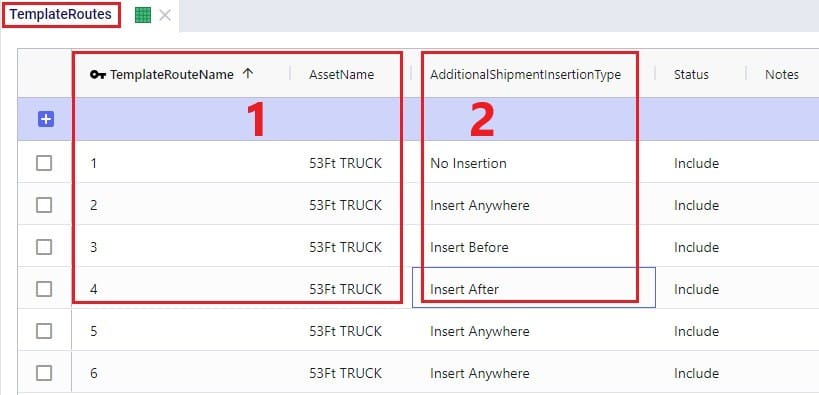
If a template route is set up by using the Template Route Name and Template Route Stop Sequence fields in the Shipments table and this route is not specified in the Template Routes table, it means that no insertions can be made into this template route.

Load Balancing Demand

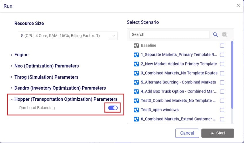
In addition to routing shipments with a fixed amount of product to be delivered to a customer location, Hopper can also solve problems where routes throughout a week need to be designed to balance out weekly demand while achieving the lowest overall routing costs. The Load Balancing Demand and Load Balancing Schedules tables can be used to set this up. If both the Shipments table and the Load Balancing Demand/Schedules tables are populated, by default the Shipments table will be used and the Load Balancing Demand/Schedules tables will be ignored. To switch to using the Load Balancing Demand/Schedules tables (and ignoring the Shipments) table, the Run Load Balancing toggle in the Hopper (Transportation Optimization) Parameters section on the Run screen needs to be switched to on (toggle to the left and grey is off; to the right and blue is on):

The weekly demand, the number of deliveries per week, and, optionally, a balancing schedule can be specified in the Load Balancing Demand table:

1. Source Name, Customer Name, and Product Name – specify the origin facility from which the product will be picked up in the Source Name field, the Customer that required the product in the Customer Name field, and the name of the product to be delivered in the Product Name field.
2. Weekly Demand – specify the weekly demand quantity (unit = eaches) this customer has for this product.
3. Number Of Deliveries Per Week – enter how often the customer needs to be delivered to per week. This field is required and when left blank the default of 1 will be used. If this number clashes with the Load Balancing Schedule used (next field), there will be unrouted shipments in the outputs.
4. Load Balancing Schedule Name – if there are other rules around how the weekly demand needs to be balanced over the week, schedules can be specified on the Load Balancing Schedules table, which will be discussed in the next section. Type the name of a Load Balancing Schedule in this field for this source-destination-product combination to use it.

Load Balancing Schedules

To balance demand over a week according to a schedule, these schedules can be specified in the Load Balancing Schedules table:

1. Load Balancing Schedule Name – the name of the load balancing schedule that is specified in this record. To use the schedule, its name needs to be used in the Load Balancing Schedule Name field of the Load Balancing Demand table.
2. Min Days and Max Days Between Delivery – if there are rules around the lower and upper limits of the number of days that are allowed in between deliveries, enter these here.
3. Monday Delivery, Tuesday Delivery, Wednesday Delivery, Thursday Delivery, Friday Delivery, Saturday Delivery, and Sunday Delivery – for each day of the week it can be specified if a delivery has to be made by setting these fields to Force, a delivery cannot be made by setting them to Prevent, or if optimal a delivery can be made by setting these fields to Consider. If nothing is specified here, the default of Consider will be used.

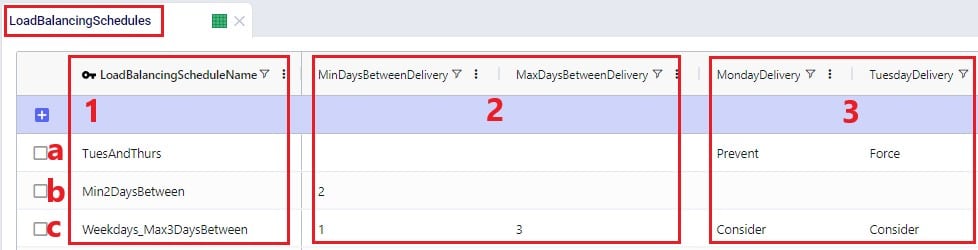
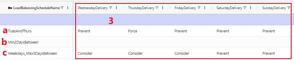
In the screenshots above, the 3 load balancing schedules that have been set up will spread the demand out as follows:

1. TuesAndThurs: this schedule forces 2 deliveries per week, 1 on Tuesday and 1 on Thursday.
2. Min2DaysBetween: this schedule allows for deliveries to be made on each day of the week, the only condition is that there are at least 2 days in between any deliveries.
3. Weekdays_Max3DaysBetween: this schedule allows for deliveries to be made on each weekday, however there cannot be more than 3 days in between any deliveries, so at least 2 deliveries per week need to be made when this schedule is used.

Relationship Constraints

In the Relationship Constraints table, we can tell Hopper what combinations of entities are not allowed on the same route. For example, in the screenshot below we are saying that customers that make up the Primary Market cannot be served on the same route as customers from the Secondary Market:

1. Entity1 and Entity2 – with these 2 entity fields we specify which entities are not allowed to be on the same route. Here Primary_Market, a Group of customers, and Secondary_Market, also a Group of customers are selected. Groups, Named Filters, and single elements can be used in these fields.
2. Entity1Type and Entity2Type – the types of entities that are disallowed to be on the same route together, here they are both set to Customer as the entities selected in the Entity1 and Entity2 fields are Groups of type = Customers. Other options are Transportation Asset, Product and Shipment.

A few examples of common Relationship Constraints are shown in the following screenshot where the Notes field explains what the constraint does:

Business Hours

To set the availability of customers, facilities, and assets to certain start and end times by day of the week, the Business Hours table can be used. The Schedule Name specified on this table can then be used in the Operating Schedule fields on the Customers, Facilities and Transportation Assets tables. Note that the Wednesday – Saturday Open Time and Close Time fields are omitted in the following screenshot:

1. Schedule Name – specify the name of the schedule that is specified in this record. Note that if a schedule has multiple time windows where it is open on the same day (say for example 9AM-12PM, and 1PM-5PM), multiple records that have the same Schedule Name can be specified in this table.
2. Sunday Open Time and Sunday Close Time – using the 24 hour clock, set the time on Sunday when the location opens or the asset becomes available in the Sunday Open Time field. Similarly, set the time on Sunday when the location closes or the asset becomes unavailable in the Sunday Close Time field. Repeat this for the Open and Close Time fields for the other days of the week. Notes:
   • If a location is closed / asset is unavailable on a certain day of the week, you should enter 0:00 as both the open and close time.
   • Leaving the open and close time fields blank means that the location is open / asset is available all day.

Business Calendars

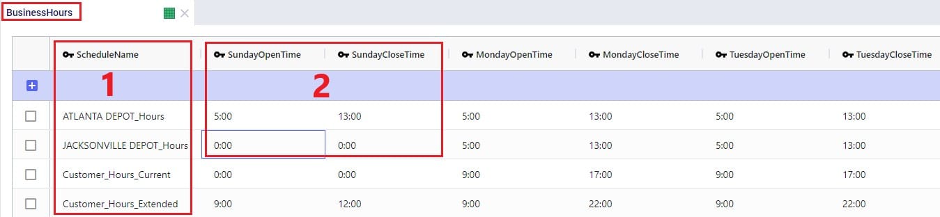
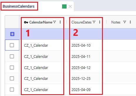
To schedule closure of customers, facilities, and assets on certain days, the Business Calendars table can be used. The Calendar Name specified on this table can then be used in the Operating Calendar fields on the Customers, Facilities and Transportation Assets tables:

1. Calendar Name – the name of the calendar, to be used in the Operating Calendar fields on the Customers, Facilities, and Transportation Assets tables. Multiple records with the same name together make up 1 calendar.
2. Closure Dates – enter the date the Customer / Facility / Asset will be unavailable. Users need to create a record for each closure date.

Groups

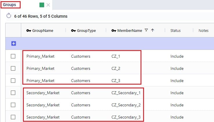
Groups are a general Cosmic Frog feature to make modelling quicker and easier. By grouping elements that behave the same together in a group we can reduce the number of records we need to populate in certain tables since we can use the Group names to populate the fields instead of setting up multiple records for each individual element which will all have the same information otherwise. Underneath the hood, when a model that uses Groups is run, these Groups are enumerated into the individual members of the group. We have for example already seen that groups of Type = Customers were used in the Relationship Constraints table in the previous section to prevent customers in the Primary Market being served on the same route as customers in the Secondary Market. Looking in the Groups table we can see which customers are part (‘members’) of each of these groups:

Examples of other Hopper input tables where use of Groups can be convenient are:

• Using a group of Facilities or Suppliers in the Domicile Location field of the Transportation Assets table to indicate that this Asset has the same characteristics in terms of cost, capacity, upper limits on distance, time and stops, and pickup & delivery times across these locations.
• Using a group of Transportation Assets in the Asset Name field of the Transit Matrix table to indicate that the Transport Distances and Transport Times set there are the same across a group of Assets.
• Using a group of Transportation Assets in the Asset Name field of the Template Routes table to indicate that the rules around insertion of additional shipments on the template route are valid across a group of Assets.
• Using groups of Customers, Shipments, Transportation Assets or Products in the Entity1 and Entity2 fields of the Relationship Constraints table to indicate that all members of the group are not allowed on the same route together with the element(s) of the other entity. E.g. groups of Chilled and Ambient products, groups of Reefer vehicles, groups of customers with access restrictions for certain groups of larger vehicles, etc.

Note that in addition to Groups, Named Filters can be used in these instances too. Learn more about Named Filters in this help center article.

Step Costs

The Step Costs table is a general table in Cosmic Frog used by multiple technologies. It is used to specify costs that change based on the throughput level. For Hopper, all cost fields on the Transportation Rates table, the Transportation Stop Rates table, and the Fixed Cost on the Transportation Assets table can be set up to use Step Costs. We will go through an example of how Step Costs are set up, associated with the correct cost field, and how to understand outputs using the following 3 screenshots of the Step Costs table, Transportation Rates table and Transportation Route Summary output table, respectively. The latter will also be discussed in more detail in the next section on Hopper outputs.

1. Step Cost Name – use this field to give the step cost structure you are setting up a unique name. All records with the same Step Cost Name (UnitCost_1 here) make up 1 set of stepped costs.
2. Step Cost Behavior – this field specifies how the stepped costs are to be applied. Options are Stepwise, Incremental and All Item:
   • Stepwise: the cost is a fixed cost up to a certain throughput level
   • Incremental: the cost is a variable cost and any discounts for higher throughputs apply from the specified throughput level only, not to all items once we go over that certain throughput.
   • All Item: the cost is a variable cost and any discounts for higher throughputs apply to all items.
3. Throughput Level – the throughput from which the specified Cost applies.
4. Cost – the cost for the throughput from this throughput level to the next throughput level applied.

In this example, the per unit cost for units 0 through 20 is $1, $0.9 for units 21 through 40, and $0.85 for all units over 40. Had the Step Cost Behavior field been set to All Item, then the per unit cost for all items is $1 if the throughput is between 0 and 20 units, the per unit cost for all items is $0.9 if the throughput is between 21 and 40 units, and the per unit cost for all items is $0.85 if the throughput is over 41 units.

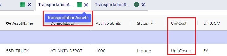
In this screenshot of the Transportation Rates table, it is shown that the Unit Cost field is set to UnitCost_1 which is the stepped cost with 3 throughput levels that we just discussed in the screenshot above:

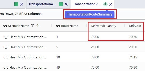
Lastly, this is a screenshot of the Transportation Route Summary output table where we see that the Delivered Quantity on Route 1 is 78. With the stepped cost structure as explained above for UnitCost_1, the Unit Cost in the output is calculated as follows: 20 * $1 (for units 1-20) + 20 * $0.9 (for units 21-40) + 38 * $0.85 (for units 41-78) = $20 + $18 + $32.30 = $70.30.

Running a Hopper Model

When the input tables have been populated and scenarios are created (several resources explaining how to set up and configure scenarios are listed in the “2.4 Status and Notes fields” section further above), one can start a Hopper run by clicking on the Run button at the top right in Cosmic Frog:

The Run screen will come up:

1. Choose the Resource Size of the solver to be used for the Hopper run.
2. In the Engine section, select Hopper.
3. In the Hopper Parameters section, optionally turn Run Load Balancing on or off. If it is off (the default) then the Shipments table will be used as the input for how much product needs to be delivered where and when, and the Load Balancing Demand & Schedules tables will be ignored. If Run Load Balancing is turned on, the Load Balancing Demand & Schedules tables will be used as the input for how much product needs to be delivered where and when, and the Shipments table will be ignored.
4. In the Scenarios list, choose the ones to run.
5. Click on the Start button to kick off the selected scenario(s).

Once a Hopper run is completed, the Hopper output tables will contain the outputs of the run.

Looking at Hopper Outputs

As with other Cosmic Frog algorithms, we can look at Hopper outputs in output tables, on maps and analytics dashboards. We will discuss each of these in the next 3 sections. Often scenarios will be compared to each other in the outputs to determine which changes need to be made to the last-mile delivery part of the supply chain.

Hopper Output Tables

In the Output Summary Tables section of the Output Tables are 8 Hopper specific tables, they start with “Transportation…”. Plus, there is also the Hopper specific detailed Transportation Activity Report table in the Output Report Tables section:

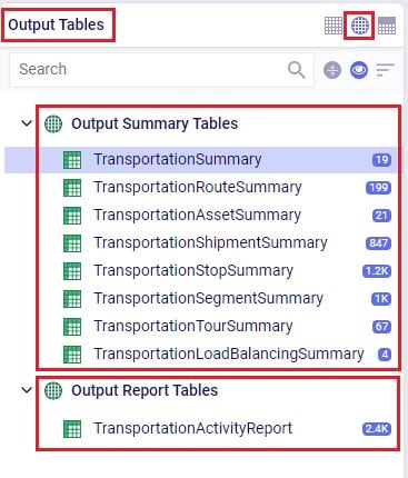
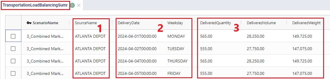
Switch from viewing Input Tables to Output Tables by clicking on the round grid at the top right of the tables list. The Transportation Summary table gives a high-level summary of each Hopper scenario that has been run and the next 6 Summary output tables contain the detailed outputs at the route, asset, shipment, stop, segment, and tour level. The Transportation Load Balancing Summary output table is populated when a Load Balancing scenario has been run, and summarizes outputs at the daily level. The Transportation Activity Report is especially useful to understand when Rests and Breaks are required on a route. All these output tables will be covered individually in the following sections.

Transportation Summary

The Transportation Summary table contains outputs for each scenario run that include Hopper run details, cost details, how much product was delivered and how, total distance and time, and how many routes, stops and shipments there were in total.

The Hopper run details that are listed for each scenario include:

• Hopper Version – the version of the Hopper algorithm that was used to run the scenario.
• Run Start Time – the date and time when the run started.
• Total Run Time – how many minutes it took to run the scenario.
• Resource Size – the size of the solver resource that was used to run the scenario.
• Consumed Memory – how much memory (in GB) was used during the Hopper solve.
• Solve Type – indicates which algorithm was run.

The next 2 screenshots show the Hopper cost outputs, summarized by scenario:

1. Total Transportation Cost – this is the total of all the costs that have been incurred in this scenario, which is the sum of the 12 cost types which are listed in the next 12 columns, plus the Total CO2 Cost which is not shown in this screenshot, and can be found farther right in this table.
2. The costs that the total transportation costs are made up of are:
   • Total Route Fixed Costs – the sum of the fixed costs associated with the routes in the scenario.
   • Total Asset Fixed Costs – the sum of all the fixed costs associated with the assets in the scenario.
   • Total Distance Cost – the sum of all the costs incurred based on how far assets travelled in the scenario.
   • Total Reposition Distance Cost – the sum of all the costs incurred based on how far assets travelled while empty in the scenario.
   • Total Out Of Route Distance Cost – the sum of all the costs incurred based on how far out of route assets travelled in the scenario.
   • Total Time Cost – the sum of all the costs incurred based on how long assets travelled in the scenario.
   • Total Wait Time Cost – the sum of all the costs incurred based on how long drivers needed to wait in the scenario.
   • Total Rest Time Cost – the sum of all the costs incurred based on how long drivers needed to rest in the scenario.
   • Total Break Time Cost – the sum of all the costs incurred based on how long drivers needed to take short breaks in the scenario.
   • Total Stop Cost – the sum of all the costs incurred based on how many stops assets made in the scenario.
   • Total Unit Cost – the sum of all the variable costs incurred based on how much product was moved in the scenario.
   • Total Direct Cost – the sum of all the direct costs incurred for serving customers directly rather than on a multi-stop route.
   • Total CO2 Cost – the sum of all the costs incurred on all routes in the scenario because of CO2 emissions.
3. Comparing scenario 2_New Market Added to Primary Template, where secondary market customers were inserted into the primary market customers’ routes, with scenario 3_Combined Markets_No Template Routes, where the routes where optimized for both primary and secondary market customers, we see that the overall cost for scenario 3 is lower which is mainly driven by much lower Distance Costs and further by lower Rest Time Costs. Based on this it seems beneficial to create entirely new routes which allow serving primary market and secondary market customers on the same route. However, there may be a cost associated with implementing these changes which will need to be taken into account in the final decision too.

Scrolling further right in the Transportation Summary table shows the details around how much product was delivered in each scenario:

For the Quantity UOM that is shown in the farthest right column in this screenshot (eaches here), the Total Delivered Quantity, Total Direct Quantity and Total Undelivered Quantity are listed in these columns. If the Total Direct Quantity is greater than 0, details around which shipments were delivered directly to the customer can be found in the Transportation Shipment Summary output table where the Shipment Status = Direct Shipping. Similarly, if the total undelivered quantity is greater than 0, then more details on which shipments were not delivered and why are detailed in the Unrouted Reason field of the Transportation Shipment Summary output table where the Shipment Status = Unrouted.

The next set of output columns when scrolling further right repeat these delivered, direct and undelivered amounts by scenario, but in terms of volume and weight.

Still further to the right we find the outputs that summarize the total distance and time by scenario:

1. Total Distance – the sum of the distances travelled by the assets on all the routes in the scenario.
2. Total Reposition Distance – the sum of the distances of the segments on all routes in the scenario where the assets were empty.
3. Total Out Of Route Distance – the sum of the out of route distances travelled by the assets on all the routes in the scenario. Out of route distance is defined in the section on the Transportation Rates table further above.
4. Total Time – the sum of the time it took for all the routes to be completed in the scenario. This is the sum of the next 5 time output columns.
5. Total Travel Time – the sum of the driving time of all the routes in the scenario.
6. Total Service Time – the sum of the time spent at locations picking up or delivering product in the scenario.
7. Total Wait Time – the sum of the time spent waiting in the scenario.
8. Total Rest Time – the sum of the time spent resting in between shifts in the scenario.
9. Total Break Time – the sum of the short breaks taken in the scenario.

Lastly, the fields furthest right on the Transportation Summary output table contain details around the number of routes, assets and shipments, and CO2 emissions:

1. Number Of Routes – the number of routes that were used in this scenario.
2. Number Of Transportation Assets – the number of vehicles (assets) that were used in this scenario.
3. Number Of Delivered Shipments – the number of shipments that were delivered to customers using a multi-stop route in this scenario.
4. Number Of Direct Shipments – the number of shipments that were delivered directly to customers in this scenario.
5. Number Of Unrouted Shipments – the number of shipments that were not delivered to customers in this scenario.
6. Total CO2 Emissions – the total amount of CO2 that was emitted during this scenario.

A few columns contained in this table are not shown in any of the above screenshots, these are:

• Total Admin Time – the sum of the total admin time spent at the start and end of routes during this scenario.
• Total CO2 Cost – the sum of all the costs incurred due to emitting CO2 for this scenario.
• Total Fuel Surcharge Cost – the sum of all the fuel surcharge costs incurred in this scenario.

Transportation Route Summary

The Transportation Route Summary table contains details for each route in each scenario that include cost, distance & time, number of stops & shipments, and the amount of product delivered on the route.

1. Route Name – the name of the route for which the details are listed here. If this is a Template Route, the name given to that Template Route in the Template Route Name field on the Shipments table will be listed here. Otherwise, if it is a Hopper generated route, the Route Name will be automatically generated and be a number, starting from 1.
2. Tour ID – a tour is defined as an asset schedule, and each tour gets assigned a unique ID, starting at 1. Routes with the same tour ID use the same asset on them. Note that this field may appear further to the right in your Transportation Route Summary table.
3. Route Start Date and Route End Date – the date and time of when the route starts at the origin location and the date and the time that the asset returns to the origin location. Note that this field may appear further to the right in your Transportation Route Summary table.
4. Origin Name – details which facility the route started from. Note that this field may appear further to the right in your Transportation Route Summary table.
5. Transportation Asset Name – details what vehicle (asset) was used for the route. Note that this field may appear further to the right in your Transportation Route Summary table.
6. Route Cost – the total cost of the route. The individual cost buckets that make up the total cost are listed in the next set of fields, see the next 2 screenshots below.
7. Route Type (not shown in the screenshot) – lists what type of route this is, possible values are:
   1. Inbound – a route with only pickup stops
   2. Outbound – a route with only delivery stops
   3. Backhaul – a route with delivery stops at the start of the route and pickup stops at the end of the route
   4. Interleaved – a route where pickup and delivery stops are mixed
   5. Template – a route that follows a template entered by the user, in other words: a fixed route where, optionally, certain types of insertions are allowed (see the Shipments and Template Routes tables how to set these up)
   6. Reposition – a route to return a vehicle to its domicile

The costs that together make up the total Route Cost are listed in the next 11 fields shown in the next 2 screenshots:

1. Fixed Cost – the one-time fixed route cost for this route, resulting from the Fixed Cost Per Route input on the Transportation Rates table.
2. Distance Cost – the cost resulting from the distance travelled on this route.
3. Reposition Distance cost – the cost incurred from the distance travelled while the asset is empty on this route.
4. Out Of Route Distance Cost – the cost incurred from the out of route distance, out of route distance is defined in the Transportation Assets table section further above.
5. Time Cost – the cost resulting from the amount of time it takes to travel on this route.
6. Wait Time Cost –the cost resulting from the amount of time the driver needed to wait on this route.
7. Rest Time Cost – the cost resulting from the amount of time the driver needed to rest on this route.
8. Break Time Cost – the cost resulting from the amount of time the driver needed to take short breaks on this route.
9. Stop Cost – the cost resulting from the amount of stops on this route.
10. Unit Cost – the variable costs incurred based on how much product was moved on this route.
11. Route CO2 Cost – the costs incurred on this route due to CO2 emissions.
12. Route Fuel Surcharge Cost (not shown in screenshot) – the costs incurred on this route as a result of fuel surcharges.

The next set of output fields show the distance and time for each route:

1. Route Distance – the total distance covered by the asset on this route. This is calculated based on the distances specified in the Transit Matrix, if populated. For segments of the route that do not have a distance specified in the Transit Matrix table, the latitudes and longitudes of the origin and destination of the segment plus the Circuity Factor set in Model Settings are used to calculate the distance.
2. Reposition Distance – the distance covered by the asset on this route while the asset is empty.
3. Out Of Route Distance – the distance of this route that is considered to be out of route based on the out of route distance definition explained in the Transportation Assets table section further above.
4. Route Time – the total time it took to complete the route. This is the sum of the times specified in the next 5 fields.
5. Route Travel Time – the total time of the route that is spent driving. This is calculated based on the times specified in the Transit Matrix table. For segments of the route that do not have a time specified in the Transit Matrix table, the time is calculated from the distance of the segment and the Speed of the asset as specified in the Transportation Assets table. If the Speed of the asset is left blank in the Transportation Assets table, then the Average Speed in the Model Settings table is used.
6. Route Service Time – the total time of the route that is spent at stops, picking up and delivering products.
7. Route Wait Time – the total time of the route that is spent waiting.
8. Route Rest Time – the total time of the route that is spent resting in between 2 shifts.
9. Route Break Time – the total time of the route that is spent on short breaks.
10. Route Admin Time (not shown in screenshot) – the total time of the route that is spent at the start and end of the route for admin purposes (e.g. paperwork).

Finally, the fields furthest right in the Transportation Route Summary table list the amount of product that was delivered on the routes, and the number of stops and delivered shipments on each route.

1. Delivered Quantity, Delivered Volume, and Delivered Weight – these list how much product was delivered on this route in terms of quantity, volume, and weight. Their UOM fields specify what the unit of measure for each of those is; here: eaches, cubic feet, and pounds.
2. Number of Stops – the number of stops made on this route.
3. Number of Delivered Shipments – the number of shipments that were delivered on this route. This can be the same number as the number of stops or it could be a higher number in case multiple shipments to the same destination were consolidated onto 1 route.
4. Route CO2 Emissions (not shown in screenshot) – the total CO2 emitted on this route.
5. Decomposition Name (not shown in screenshot) – the decomposition name given to the shipments on this route (Decomposition Name input field on the Shipments table).

Transportation Asset Summary

The Transportation Asset Summary output table contains the details of each type of asset used in each scenario. These details include costs, amount of product delivered, distance & time, and the number of delivered shipments.

1. Transportation Asset Name, Origin Name, Number Used – detail how often this asset type was used starting at this facility/supplier during this scenario.
2. Total Cost – the total cost for this asset type starting from this origin during the scenario. The individual cost buckets are listed in the next several fields, see the next screenshot below.

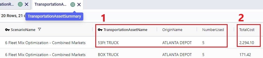
The costs that together make up the Total Cost are listed in the next 12 fields:

1. Total Route Fixed Cost – the total of the one-time costs applied on each route for this asset type (resulting from the Fixed Cost Per Route input on the Transportation Rates table).
2. Total Fixed Cost – the total of the one-time asset costs for this asset type (resulting from the Fixed Cost input on the Transportation Assets table).
3. Total Distance Cost – the total of the costs resulting from the distance travelled by this asset type.
4. Total Reposition Distance Cost – the total of the costs resulting from the distance travelled by this asset type while empty.
5. Total Out Of Route Distance Cost – the total of the costs incurred from the out of route distance travelled by this asset type; out of route distance is defined in the Transportation Assets table section further above.
6. Total Time Cost – the total of the costs resulting from the amount of time this asset type was used.
7. Total Wait Time Cost – the total of the costs resulting from the amount of time this asset type has needed to wait on the routes it was used on.
8. Total Rest Time Cost – the total of the costs resulting from the amount of time this asset type has needed to rest in between 2 shifts on the routes it was used on.
9. Total Break Time Cost – the total of the costs resulting from the amount of time this asset type has needed to take short breaks on the routes it was used on.
10. Total Stop Cost – the total of the costs resulting from the cost per stop for all the stops this asset type made on the routes it was used on.
11. Total Unit Cost – the total of the variable costs resulting from the amount of product this asset type delivered on the routes it was used on.
12. Total CO2 Cost – the total of the costs resulting from the CO2 emitted by this asset type on the routes it was used on.
13. Total Fuel Surcharge Cost – the total of the costs resulting from applying a fuel surcharge to this asset type on the routes it was used on.

The next set of fields in the Transportation Asset Summary summarize the distances and times by asset type for the scenario:

1. Total Distance – the total distance covered by this asset type on the routes it is used on. See the notes on the Route Distance field in the Transportation Route Summary on how distances are calculated.
2. Total Reposition Distance – the total distance covered by this asset type on the routes it is used on while empty.
3. Total Out Of Route Distance – the total distance that is considered out of route for this asset type on the routes it is used on. See the section on the Transportation Assets table for the definition of Out Of Route Distance.
4. Total Time – the total time it took to complete the routes this asset type is used on.
5. Total Travel Time – the total driving time for this asset type on the routes it is used on. See the notes on the Route Time field in the Transportation Route Summary on how times are calculated.
6. Total Service Time – the total time for this asset type that is spent at stops, picking up and delivering products, on the routes it is used on.
7. Total Wait Time – the total time for this asset type that is spent waiting on the routes it is used on.
8. Total Rest Time – the total time for this asset type that is spent resting in between 2 shifts on the routes it is used on.
9. Total Break Time – the total time for this asset type that is spent on short breaks on the routes it is used on.
10. Total Admin Time (not shown in screenshot) – the total time for this asset type that is spent doing admin (e.g. paperwork) at the start and end of routes it is used on.

Furthest to the right on the Transportation Asset Summary output table we find the outputs that list the total amount of product that was delivered, the number of delivered shipments, and the total CO2 emissions:

1. Total Delivered Quantity, Total Delivered Volume, and Total Delivered Weight – these list how much product in total was delivered by this asset type on the routes it is used on in terms of quantity, volume, and weight. Their UOM fields specify what the unit of measure for each of those is; here: eaches, cubic feet, and pounds.
2. Number of Delivered Shipments (not shown in screenshot) – the number of shipments that were delivered by this asset type on the routes it is used on.
3. Total CO2 Emissions (not shown in screenshot) – the total CO2 emitted by this asset type on the routes it is used on.

Transportation Shipment Summary

The Transportation Shipment Summary output table lists for each included Shipment of the scenario the details of which asset type it is served by, which stop on which route it is, the amount of product delivered, the allocated cost, and its status.

1. Shipment ID – the ID of the Shipment as specified in the Shipments input table. In case a Load Balancing Demand scenario has been run (see Load Balancing Demand input table further above for details on how to set this up and run this), the Shipment ID will be autogenerated by Hopper.
2. Transportation Asset Name – the vehicle type (asset) the shipment is served by.
3. Source Name, Destination Name, Product Name – the location (source) from which the customer (destination) is served, and the name of the product that is delivered.
4. Route Name – the name of the route this Shipment is on. If this is a Template Route, the name given to that Template Route in the Template Route Name field on the Shipments table will be listed here. Otherwise, if it is a Hopper generated route, the Route Name will be automatically generated and be a number, starting from 1.
5. Stop ID – the destination’s stop number on the route. If this stop is on a Template Route, the Stop ID will be the same as the number in the Template Route Stop Sequence field on the Shipments table if no insertions of other Shipments were made. If insertions were allowed and also made, the Stop ID field may be different.
6. Route Type (not shown in screenshot) – the type of route this shipment is on. Possible values are: Inbound, Outbound, Backhaul, Interleaved, Template, and Reposition. For more details see description further above of the Route Type field in the Transportation Route Summary output table section.

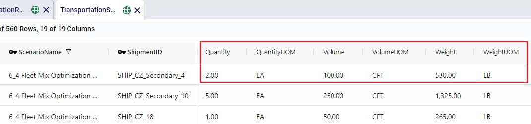
The next set of fields in the Transportation Shipment Summary table list the total amount of product that was delivered to this stop.

• Quantity, Volume, and Weight – these list how much product of this shipment was delivered by this asset type in terms of quantity, volume, and weight. Their UOM fields specify what the unit of measure for each of those is; here: eaches, cubic feet, and pounds.

The next screenshot of the Transportation Shipment Summary shows the outputs that detail the status of the shipment, costs, and a reason in case the shipment was unrouted.

1. Shipment Status – this will show 1 of 3 possible statuses of the Shipment:
   • Routed: the Shipment was delivered as part of a multi-stop route.
   • Direct Shipping: the Shipment was delivered directly and not as part of a multi-stop route.
   • Unrouted: the Shipment has not been delivered.
2. Allocated Route Cost and Allocated Route Cost Percent – the portion of the cost of the route the shipment is responsible for in absolute and percentage of total route cost.
3. Direct Cost – if the Shipment was delivered directly, this field shows the cost associated with that direct shipping.
4. Unrouted Reason – if the Shipment Status of the Shipment = Unrouted, the reason why the Shipment could not be routed will be given here.

Lastly, the outputs furthest to the right on the Transportation Shipment Summary output table list the pickup and delivery time and dates, the allocation of CO2 emissions and associated costs, and the Decomposition Name if used:

1. Pickup Date – the date and time when the product of the shipment was picked up from its origin location. This date and time are the start of the service time at that location, which can be the same as or later than the arrival time at this location.
2. Delivery Date – the date and time when the product of the shipment was delivered to its destination location. This date and time are the start of the service time at that location, which can the same as of later than the arrival time at this location.
3. Allocated CO2 Emissions and Allocated CO2 Cost – the CO2 emissions that this shipment is responsible for and the cost associated with them.
4. Decomposition Name – the decomposition name given to the shipment in the Shipments table.

Transportation Stop Summary

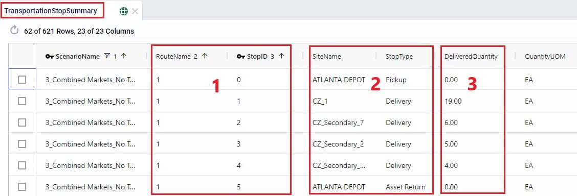
The Transportation Stop Summary output table lists for each route all the individual stops and their details around amount of product delivered, allocated cost, service time, and stop location information.

‍

This first screenshot shows the basic details of the stops in terms of route name, stop ID, location, stop type, and how much product was delivered:

1. Route Name and Stop ID – the name of the route the Stop is on and the number of the stop on this route. The facility location that the shipments are delivered from is the first stop and is given Stop ID 0 so that the first stop with Stop ID 1 is the destination of a Shipment where product is delivered to.
2. Site Name and Stop Type – the location name of the Stop, which can be a facility, or customer and the Stop Type, which can be Pickup, Delivery or Asset Return.
3. Delivered Quantity, Delivered Volume (not shown in screenshot), and Delivered Weight (not shown in screenshot) – these list how much product was delivered to this stop on this route in terms of quantity, volume, and weight. Their UOM fields specify what the unit of measure for each of those is.
4. Route Type (not shown in screenshot) – the type of route this stop is on. Possible values are: Inbound, Outbound, Backhaul, Interleaved, Template, and Reposition. For more details see description further above of the Route Type field in the Transportation Route Summary output table section.

Somewhat further right on the Transportation Stop Summary table we find the outputs that detail the route cost allocation and the different types of time spent at the stop:

1. Allocated Route Cost and Allocated Route Cost Percent – the portion of the cost of the route the stop is responsible for in absolute and percentage of total route cost.
2. Service Time – the time the vehicle spends in total at this stop. The inputs into Service time are the fixed and unit pickup and delivery times specified on the Shipments, Transportation Assets, Customers, and Facilities tables.
3. Wait Time – the time the vehicle spent waiting at this stop, for example if it arrives before the stop is open.
4. Rest Time – the time the vehicle spent resting in between 2 shifts at this stop.
5. Break Time – the time the vehicle spent on short break at this stop.
6. Admin Time (not shown in screenshot) – the time the vehicle spent as admin time at this stop.

Lastly, farthest right on the Transportation Stop Summary table, arrival, service, and departure dates are listed, along with the stop’s latitude and longitude:

1. Arrival Date – the date and time the vehicle arrives at this stop.
2. Service Date – the date and time the vehicle starts service at this stop.
3. Departure Date – the date and time the vehicle leaves this stop.
4. Latitude and Longitude – the latitudes and longitudes of the stops are repeated here from the input tables (from the Facilities or Customers input table).

Transportation Segment Summary

The Transportation Segment Summary output table contains distance, time, and source and destination location details for each segment (or “leg”) of each route.

The basic details of each segment are shown in the following screenshot of the Transportation Segment Summary table:

1. Route Name and Segment ID – the name of the route and the number of the segment on the route.
2. Origin Name and Destination Name – the location where the segment starts from (origin) and the location where the segment ends at (destination).
3. Segment Distance – the distance of the segment. See the notes on the Route Distance field in the Transportation Route Summary on how distances are calculated.
4. Route Type (not shown in screenshot) – the type of route this segment is on. Possible values are: Inbound, Outbound, Backhaul, Interleaved, Template, and Reposition. For more details see description further above of the Route Type field in the Transportation Route Summary output table section.
5. Tour ID (not shown in screenshot) – the tour (= asset schedule) that this segment is part of.

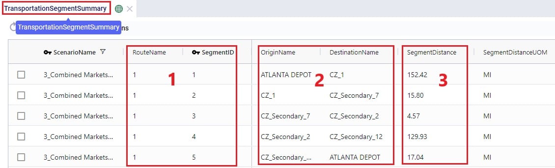
Further right on the Transportation Segment Summary output table, the time details of each segment are shown:

1. Segment Time – the total time this segment takes, which is the sum of the next 3 time output fields.
2. Segment Travel Time – the time it takes to travel the segment. See the notes on the Route Time field in the Transportation Route Summary on how times are calculated.
3. Segment Rest Time – the total rest time in between shifts that was taken on this segment of the route.
4. Segment Break Time – the total short break time that was taken on this segment of the route.

Next on the Transportation Segment Summary table are the latitudes and longitudes of the segment’s origin and destination locations:

1. Origin Latitude and Origin Longitude – the latitude and longitude of the segment’s origin location are repeated here (from the facilities or Customers input table).
2. Destination Latitude and Destination Longitude – the latitude and longitude of the segment’s destination location are repeated here (from the Facilities or Customers input table).

And farthest right on the Transportation Segment Summary output table details around the start and end date and time of the segment are listed, plus CO2 emissions and the associated CO2 cost:

1. Start Date – the time and date when the asset leaves the segment’s origin location.
2. End Date – the time and date when the arrives at the segment’s destination location.
3. CO2 Emissions and CO2 Cost – the CO2 emitted by the asset on this segment of the route and the cost associated with it.

Transportation Tour Summary

For each Tour (= asset schedule) the Transportation Tour Summary output table summarizes the costs, distances, times, and CO2 details.

The next 3 screenshots show the basic tour details and all costs associated with a tour:

1. Tour ID – the unique identifier of the tour within the scenario.
2. Transportation Asset Name and Origin Name – the type of transportation asset (vehicle) used on the tour and the location from where the routes within the tour start.
3. Number Of Routes – the number of routes on this tour.
4. Tour Cost – the total cost associated with this tour, this is the sum of the next 11 cost fields.
5. Tour Route Fixed Cost – the costs resulting from the fixed cost that is applied once to each route within the tour.
6. Tour Asset Fixed Cost – the costs resulting from the fixed cost that is applied once to the asset used for this tour.
7. Tour Distance Cost – the costs resulting from the total distance travelled by this asset on this tour.
8. Tour Reposition Distance Cost – the costs resulting from the distance travelled by this asset while empty on this tour.
9. Tour Out Of Route Distance Cost – the costs resulting from the distance travelled that is considered out of route by this asset on this tour. The definition of Out Of Route Distance is explained in the Transportation Assets section further above.
10. Tour Time Cost – the costs resulting from the total time the tour takes.
11. Tour Wait Time Cost – the costs resulting from the amount of time the asset had to wait while on this tour.
12. Tour Rest Time Cost – the costs resulting from the rests in between shifts that were taken while on this tour.
13. Tour Break Time Cost – the costs resulting from the short breaks that were taken while on this tour.
14. Tour Stop Cost – the total costs for all stops on the routes of this tour.
15. Tour Unit Cost – the costs resulting from the amount of product moved while on this tour.
16. Tour Fuel Surcharge Cost (not shown in screenshot) – the costs resulting from applying a fuel surcharge to the routes of this tour.

The next screenshot shows the distance outputs available for each tour on the Transportation Tour Summary output table:

1. Tour Distance – the total distance of the routes of the tour together.
2. Tour Reposition Distance – the total distance of the routes of the tour together where the asset was empty.
3. Tour Out Of Route Distance – the total distance that is considered to be out of route for the entire tour. Out Of Route Distance is explained in the Transportation Asset section further above.

Scrolling further right on the Transportation Tour Summary table, the outputs available for tour times are listed:

1. Tour Time – the total time the routes of the tour take.
2. Tour Travel Time – the total drive time of the tour.
3. Tour Service Time – the total time spent servicing the stops on all routes of the tour, picking up and delivering products.
4. Tour Wait Time – the total time spent waiting on the tour.
5. Tour Rest Time – the total rest spent in between shifts on the routes of the tour together.
6. Tour Break Time – the total time spent on short breaks on the routes of the tour together.
7. Tour Admin Time (not shown in screenshot) – the total time spent on admin (e.g. paperwork) at the start and end of the routes of the tour together.

1. Tour Start Date – the date and time when the first route in the tour starts.
2. Tour End Date – the date and time when the last route in the tour finishes.
3. Tour CO2 Emissions and Tour CO2 Cost – the total CO2 emitted on the routes of the tour together and the cost associated with these CO2 emissions.
4. Decomposition Name – the decomposition name given to the shipments of this tour in the Shipments table.

Transportation Load Balancing Summary

If a load balancing scenario has been run (see the Load Balancing Demand input table further above for more details on how to run this), then the Transportation Load Balancing Summary output table will be populated too. Details on amount of product delivered, plus the number of routes, assets and delivered shipments by day of the week can be found in this output table; see the following 2 screenshots:

1. Source Name – the origin location for the routes on this day of the week.
2. Delivery Date and Weekday – the date and time from which the routes start and which day of the week this is.
3. Delivered Quantity, Delivered Volume, and Delivered Weight (UOM fields omitted in screenshot) – how much product is delivered on this day of the week from this source, in terms of quantity, volume, and weight.

1. Total Distance – the total distance of all routes from this source on this day of the week.
2. Total Time – the total time it takes for the routes to be completed from this source on this day of the week.
3. Number Of Routes – how many routes are being completed from this source on this day of the week.
4. Number Of Transportation Assets – how many assets are needed to complete all routes from this source on this day of the week.
5. Number Of Delivered Shipments – the number of shipments completed on all routes from this source on this day of the week.

Transportation Activity Report

For each route, the Transportation Activity Report details all the activities that happen in chronological order with details around distance and time and it breaks down how far along the duty and drive times are at each point in the route, which is very helpful to understand when rests and short breaks are happening.

‍

This first screenshot of the Transportation Activity Report shows the basic details of the activities:

1. Activity ID – the unique ID of the activity on the route. Automatically generated by Hopper, starting from 1.
2. Type – the type of activity this record concerns, which will be one of:
   • Pickup: when starting a route at the origin location of a route where it picks up product and at stops where product is being picked up
   • Travel: when the asset is en route from the start location to the end location of the activity
   • Delivery: when product is delivered to a stop
   • Vehicle Return: when the asset returns back to its domicile location
   • Wait: when the asset is waiting somewhere
   • Break: when the driver is on a break
   • Rest: when the driver is taking a rest
   • Admin: when admin (e.g. paperwork) is performed, which can be configured to be done at the start and/or end of a route
3. Start Date and End Date: the date and time of when the activity starts and the date and time of when the activity ends.
4. Route Name – the name of the route the current activity happens on.
5. Transportation Asset Name – the name of the asset used on this route.
6. Start Location Name and End Location Name – where the activity starts and where it ends. For Pickup, Delivery, and Vehicle Return these 2 locations are the same.
7. Route Type (not shown in screenshot) – the type of route this activity is part of. Possible values are: Inbound, Outbound, Backhaul, Interleaved, Template, and Reposition. For more details see description further above of the Route Type field in the Transportation Route Summary output table section.
8. Tour ID (not shown in screenshot) – the tour (= asset schedule) that this activity is part of.

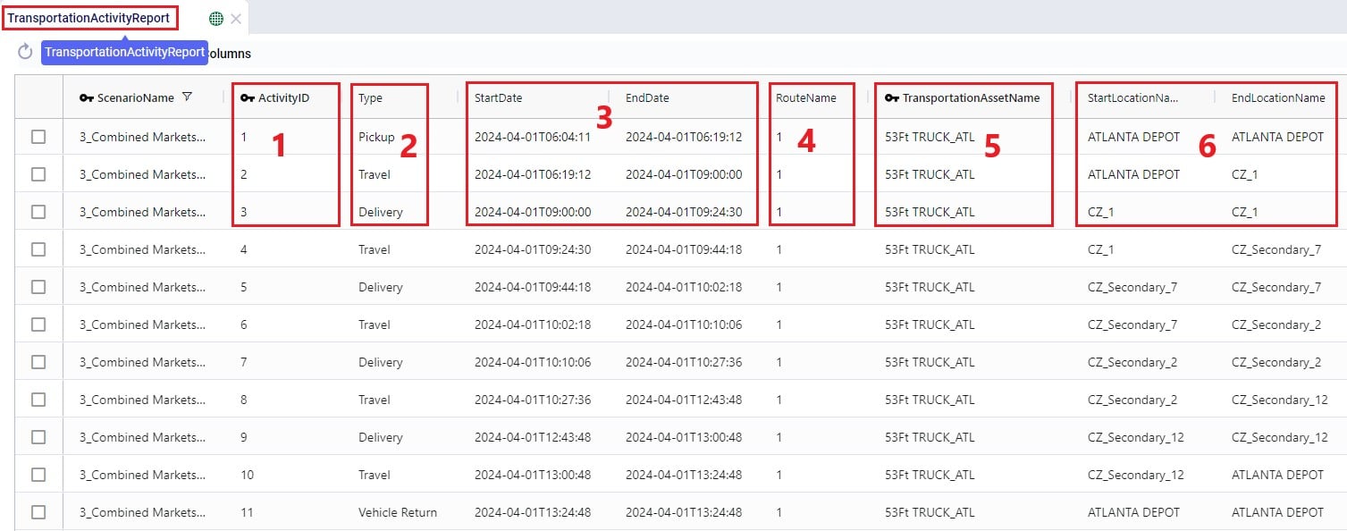
Next, the distance, time, and delivered amount of product are detailed on the Transportation Activity Report:

1. Distance – the distance of the activity. Where the activity’s start and end locations are the same, the distance is 0.
2. Time – the time the activity takes.
3. Quantity, Volume (not shown in screenshot), and Weight (not shown in screenshot) and their associated UOM fields – the amount of product that is being picked up for an activity of Type Pickup or the amount of product that is being delivered for an activity of Type Delivery; these are in terms of quantity, volume, and weight, respectively.
4. Pickup Quantity, Pickup Volume, and Pickup Weight (all 3 not shown in screenshot above) – the amount of product that is being picked up as part of this activity, in terms of quantity, volume, and weight, respectively.
5. Delivered Quantity, Delivered Volume, and Delivered Weight (all 3 not shown in screenshot above) – the amount of product that is being delivered as part of this activity, in terms of quantity, volume, and weight, respectively.

Finally, the last several fields on the Transportation Activity Report details cost, and the thus far accumulated duty and drive times:

1. Activity Cost – the cost associated with the activity.
2. Current Duty Time Within Shift – the cumulative duty time of all activities on the route so far. Once this reaches the Max Duty Time Within Shift (specified in the Transportation Assets table) this will trigger a Rest (of length Rest Time Between Shifts, also specified in the Transportation Assets table).
3. Current Drive Time Within Shift – the cumulative drive time of all travel activities on the route so far. Once this reaches the Max Drive Time Within Shift (specified in the Transportation Assets table) this will trigger a Rest (of Length Rest Time Between Shifts, also specified in the Transportation Assets table).
4. Current Drive Time Before Short Break – the cumulative drive time of all activities on the route so far. Once this reaches the Max Drive Time Before Short Break (specified in the Transportation Assets table) this will trigger a Short Break (of length Short Break Time, also specified in the Transportation Assets table).

Hopper Maps

As with the other engines within Cosmic Frog, Maps are very helpful in visualizing baseline and scenario outputs. Here, we will discuss how to set up Hopper specific Maps at a high level; we will not cover all the ins and outs of maps. If you are unfamiliar with the Maps module in Cosmic Frog, then please review the “Getting Started with Maps” article in the Optilogic Help Center first. It covers how to add and configure new maps and their layers.

Visualizing Hopper routes and direct shipments on maps is achieved by adding map layers which use 1 of the following as the table name:

• A Hopper output table, these 4 are currently available:
  
  • Transportation Stop Summary - for example use this to style stops based on the delivered / picked up quantity using breakpoints or to show only stops from (a) certain route(s) or to
  • Transportation Segment Summary - for example use this to show or style route segments based on their distance or travel time, either by using the condition builder to filter (e.g. segmentdistance > 100) or using breakpoints
  • Transportation Shipment Summary - for example use this to show unrouted shipments or those going direct (e.g. condition builder filter of shipmentstatus = 'Unrouted' or shipmentstatus = 'Direct Shipping')
  • Transportation Territory Assignment Summary - in models that use the Territory Planning feature, this table can be used to show and style stops that belong to specific territories (e.g. condition builder filter of territory name = '3' or territory type = 'Small Territories')
• The Transportation Routes Map Layer - a view created from the Transportation Segment Summary and Transportation Route Summary output tables, specifically for visualization of routes. This view is not visible in the Data module. As it contains a lot of information by segment and of the route the segment is on, using this as the table to draw the routes from gives users a lot of options for filtering and styling the routes. Plus, additional information about the segment or route can be shown in tooltips or labels.

‍

‍

Using what we have discussed above and the learnings from the Getting Started with Maps help center article, we can create the following map quite easily and quickly (the model used here is one from the Resource Library, named Transportation Optimization):

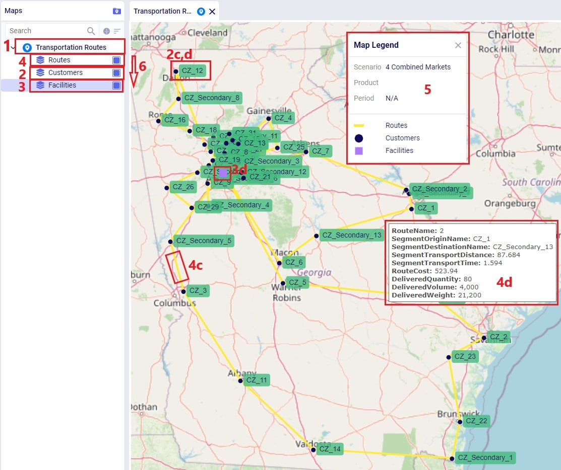
The steps taken to create this map are:

1. Use Map > New Map to add a new map:
   1. Type the name for the map: “Transportation Routes”.
   2. In the Map Filters view on the right-hand side of the map, select scenario “4 Combined Markets”.
2. While the Transportation Routes map is selected in the Maps list choose Map > New Layer:
   1. Type the name for the layer: “Customers”.
   2. In the Condition Builder view on the right hand-side of the map, choose Customers from the Table Name drop-down.
   3. Switch to the Layer Style view on the right-hand side of the map and use the defaults of blue black circles of size 6 and 100% opacity.
   4. Switch to the Layer Labels view on the right-hand side of the map and configure the labels to show CustomerName (choose this from the Labels drop-down list), keep the defaults for color (Blue Black), Size (14), Font (Arial, sans-serif), Background (on and Pale Green color), change Position to Right, and no fields for the tooltip were selected.
3. While the Transportation Routes map is selected in the Maps list choose Map > New Layer:
   1. Type the name for the layer: “Facilities”.
   2. In the Condition Builder view on the right hand-side of the map, choose Facilities from the Table Name drop-down.
   3. In the Condition Builder view on the right hand-side of the map, type “status = ‘Include’” (without the double quotes) in the Conditions text field to only show the included ATLANTA DEPOT on the map and not the excluded JACKSONVILLE DEPOT.
   4. Switch to the Layer Style view on the right-hand side of the map and change the Shape to Square, the Color to Violet and the Size px to 12.
4. While the Transportation Routes map is selected in the Maps list choose Map > New Layer
   1. Type the name for the layer: “Routes”.
   2. In the Condition Builder view on the right hand-side of the map, choose TransportationRoutesMapLayer from the Table Name drop-down.
   3. Switch to the Layer Style view on the right-hand side of the map and change the Color to Yellow, otherwise keep the default settings.
   4. Switch to the Layer Labels view on the right-hand side of the map and select the following fields in the Tooltips section (and in this order to match the above screenshot): Route Name, Segment Origin Name, Segment Destination Name, Segment Transport Distance, Segment Transport Time, Route Cost, Delivered Quantity, Delivered Volume, Delivered Weight.
5. Select the Transportation Routes map in the Maps list and switch to Map Legend in the view on the right-hand side of the map. Enable all checkboxes here to show the Legend on the map and all possible items.
6. Click on the Facilities layer and drag it down so it is the last layer in the Transportation Routes map. Do the same for the Customers layer and position it above the Facilities layer. The layers are drawn on the map in the order they are listed, so this way the Facilities layer will be shown on top, and the violet square of ATLANTA DEPOT will not be covered by the blue black customer circles, the customer labels, or the yellow route lines.
7. Zoom the map to your desired level using the plus and minus icons at the top right of the map (not shown in the screenshot above).

Let’s also cover 2 maps of a model where both pickups and deliveries are being made, from “backhaul” and to “linehaul” customers, respectively. When setting the LIFO (Is Last In First Out) field on the Transportation Assets table to True, this leads to routes that contain both pickup and delivery stops, but all the pickups are made at the end (e.g. modeling backhaul):

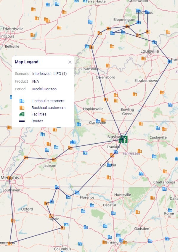
Two example routes are being shown in the screenshot above and we can see that all deliveries are first made to the linehaul customers which have blue icons. Then, pickups are made at the backhaul customers which have orange icons. If we want to design interleaved routes where pickups and deliveries can be mixed, we need to set the LIFO field to False. The following screenshot shows 2 of these interleaved routes:

The above 2 screenshots use the Transportation Routes Map Layer as the table name to draw the Routes map layer, where the condition builder is used to filter for 2 of the route names.

Finally, we will go back to the Transportation Optimization model which was used for the first map screenshot in this section. The Baseline scenario in this model has 1 shipment that is being shipped directly. To visualize this on the map we add a map layer named "Direct Shipping" which uses the Transportation Shipment Summary as the table name input. On the Layer Style pane we change the color for this line layer to red. We also keep the "Routes" map layer, which is drawn from the Transportation Routes Map Layer with the default dark blue color:

Hopper Analytics

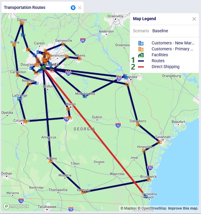
In the Analytics module of Cosmic Frog, dashboards that show graphs of scenario outputs, sliced and diced to the user’s preferences, can quickly be configured. Like Maps, this functionality is not Hopper specific and other Cosmic Frog technologies use these extensively too. We will cover setting up a Hopper specific visualization, but not all the details of configuring dashboards. Please review these resources on Analytics in Cosmic Frog first if you are not yet familiar with these:

• Optilogic Help Center article “Getting Started With Analytics”
• Optilogic Help Center article “Editing Dashboards and Visualizations”
• “Analytics Overview” video
• Training Session “Scenario Creation and Maps and Analytics”

We will do a quick step by step walk through of how to set up a visualization of comparing scenario costs by cost type in a new dashboard:

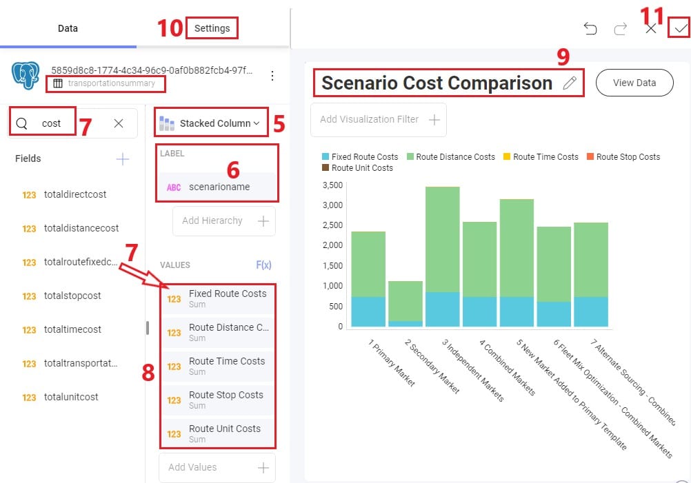
The steps to set this up are detailed here, note that the first 4 bullet points are not shown in the screenshot above:

1. In the drop-down of the Module Menu, select Analytics.
2. Click on Analytics > New Dashboard, type the name of your dashboard, for example “Transportation Scenario Comparison”, and click Done.
3. Click on “+ Visualization” in the right top corner of the new dashboard.
4. Stay in the Tables section of the Set up the Database dialogue and start typing “transportationsummary” in the search box, select the transportationsummary table by checking the circular checkbox, and click on Select Data at the bottom.
5. At the right top of the Data configuration window on the left click on the Chart Type drop-down, which shows “Column” by default to choose a chart type. For this scenario comparison, we will select Stacked Column.
6. Drag scenarioname from the fields list on the left on top of the Add Label field on the right.
7. Type “cost” in the search box at the top left of the configuration window and then drag all fields, except for total direct cost and total transportation cost, one by one on top of the of Add Values field on the right.
8. Click on the cost fields that are now in the Values section on the right to update any field settings: rename them by clicking on the pencil icon next to the name, and adjust any of the aggregation, sorting, etc. settings as desired. When finished click on Update Field at the bottom.
9. The name of the visualization is showing as transportationsummary based on the table it is derived from, this can be changed by clicking on the pencil icon next the name above the graph. We have renamed it to Scenario Cost Comparison here.
10. Before finalizing the visualization, click on the Settings tab to review if any updates need to be made here. One can choose to show the visualization’s title, legend, tooltips, etc.
11. Click on the check icon at the top right of the graph configuration window to save this visualization.
12. Now you can choose to add another visualization to this same dashboard by clicking on “+ Visualization” or if the dashboard contains all desired visualizations at this point, you can click on the check icon at the right top of the dashboard.

Available Resources for Hopper

All Hopper specific Help Center articles can be found in the Hopper - Transportation Optimization section under Navigating Cosmic Frog.

There are also several models in the Resource Library that transportation optimization users may find helpful to review. How to use resources in the Resource Library is described in the help center article “How to Use the Resource Library”.

• The Resource Library Cosmic Frog model named “Transportation Optimization” explores template routes, optimized routes, fleet mix, adding additional customers, introducing a new asset type, and adding an alternative source facility. This Transportation Optimization Template YouTube video also showcases this model.
• The Resource Library Cosmic Frog model named “Multi Stop Routes with Time Windows” extends the model from the previous bullet with features such as Business Hours, Shipment Pickup & Delivery Windows, Drive Time Regulations, and Fleet Optimization.
• The Resource Library Cosmic Frog model named “UK Multi Drop Fleet Optimization” shows the optimization of fleet mix of different vehicle types across multi-stop routes. Different vehicle types suited for Chilled vs Ambient product are available, and access restrictions at certain customers due to vehicle size are considered. A new vehicle type that can carry both Ambient and Chilled product is added to the vehicle mix in a scenario as well.
• The Resource Library Cosmic Frog model named “United States Distribution and Logistics” shows an example of how Neo (network optimization) and Hopper (transportation optimization) can be used together to optimize both the supply chain structure and asset/carrier transportation.
• The Resource Library Cosmic Frog model named “Hop Through Model” serves as a comprehensive guide to help users navigate the Hop Through exercise. In this exercise users can enhance their ability to create strategic scenarios, build insightful maps, and develop interactive dashboards. Part of this exercise is Hopper focused.

‍

Overview

Incremental Change is a powerful new capability in Cosmic Frog’s NEO engine (Network Optimization) that helps you manage the transition between two network states – such as moving from your current baseline network to an optimized future state. Rather than implementing all changes at once, Incremental Change allows you to control the pace and sequence of changes over time, making network transformations more practical and manageable.

This feature bridges the gap between theoretical optimization results and realistic implementation plans by generating a sequenced roadmap of network changes.

In this documentation, we will discuss the impact of Incremental Change, explain how to use it, and then walk through 2 demo models showing examples of the new capabilities. These models can be copied to your own Optilogic account from the Resource Library:

• Example model 1: Incremental Change - Production Smoothing
• Example model 2: Incremental Change - Supplier Base Transition

Please also see the following brief video for an introduction to Incremental Change and an overview of the second demo model, Incremental Change - Supplier Base Transition:

Why It Matters

Supply chain networks rarely change overnight. Whether you are opening new distribution centers, shifting supplier bases, or adapting to seasonal demand fluctuations, real-world constraints limit how quickly you can implement changes. Organizations face practical limitations including:

• Operational capacity - You can only onboard a limited number of new customers or suppliers per month
• Financial constraints - Capital investments must be spread across budget cycles
• Risk management - Gradual transitions reduce disruption and allow for course corrections
• Seasonal variability - Production and demand patterns require stability within acceptable ranges

Incremental Change addresses these realities by helping you answer critical questions: What is the best order of changes? What is the optimal rate of change? What tolerance levels are appropriate for different types of modifications?

Key Benefits

1. Identify High-Impact Changes

Understand which network modifications deliver the greatest value earliest in your transition. Incremental Change provides clear visibility into expected savings versus the number of changes required, along with detailed change checklists for each scenario.

2. Build Practical Transition Plans

Create realistic, step-by-step roadmaps for moving from your current network to your target network. You will receive:

• Period-by-period change checklists
• Expected transition timelines
• Monthly cost projections throughout the transition window

3. Adapt Smoothly to Dynamic Environments

Manage network evolution in response to changing business conditions while respecting operational constraints. Balance total cost optimization against your tolerance for change, with detailed monthly implementation plans.

Supported Change Types

Cosmic Frog's Incremental Change currently supports the following network changes:

• Facilities Opened – Number of new facilities added
• Facilities Closed – Number of existing facilities removed
• Suppliers Added – Number of new suppliers introduced
• Suppliers Removed – Number of existing suppliers discontinued
• Production Increase – Total production increase across all products and facilities
• Production Decrease – Total production decrease across all products and facilities
• Lanes Added – Number of new transportation lanes utilized

Practical Applications

Progressive Facility Expansion: When opening a new distribution center, specify that you want to reassign up to 10 customers per month, and the system determines which customers to transition each month to maximize savings.

Seasonal Production Smoothing: For products with seasonal demand patterns, set constraints to ensure facility production never varies by more than 10% month-over-month, maintaining operational stability.

Multi-Year Facility Rollouts: Plan the optimal sequence for opening 10 facilities over five years including a detailed 2-year implementation roadmap.

Strategic Supplier Transitions: Systematically shift your supplier base. For example, progressively move sourcing out of or into a particular region – with Incremental Change determining the optimal sequence of supplier changes.

How to Use

Incremental Change uses a new input table and generates 2 new output tables with different levels of detail:

Input: Use the Incremental Change Constraints table to set the change type(s) being included and your change budget for each period.

Outputs:

• Optimization Incremental Change Summary - Overview of the amount of change occurring in each period
• Optimization Incremental Change Report - Detailed information about each specific change taking place

By leveraging Incremental Change, you can transform theoretical network optimization results into actionable, phased implementation plans that respect real-world operational constraints while maximizing value delivery.

Tips & Tricks

Some additional pointers that may prove helpful are as follows:

• You can initially setup any Incremental Change Constraints with a large budget. This may not impose any actual limits, but it will show you the Incremental Change Outputs and can give additional direction on how to limit the changes.
• Different change types can be used in the same model / scenario.
• If no change has happened, the Optimization Incremental Change Report output table will be empty, but the Optimization Incremental Change Summary output table will show the zero change amount(s)/count(s).
• Users are encouraged to check outputs to ensure the desired behavior is achieved. If not, the most common solution is to add additional constraints to eliminate any undesired behavior.
  • For example, requiring at least 2 suppliers for 1 product can lead to the cheapest supplier being used for almost all units and only using the second cheapest supplier for a few units. Adding (conditional) minimum flow constraints can resolve this.
• Important: the Period Name Group Behavior field on the Incremental Change Constraints table always uses the Enumerate value, regardless of the value it is set to.

Example Model 1 – Production Smoothing

In this example model, "Incremental Change - Production Smoothing", we will see how we can ensure that increases in production from one month to the next are limited to a certain percentage using the Incremental Change feature. This model can be copied from the Resource Library to your own account in case you want to follow along.

Production Smoothing – Inputs

The following screenshot shows which input tables are populated in this example model:

1. We have used the Module menu to open the Data module.
2. Input tables are being shown in the list; use the left most of the 3 icons to show input tables. Clicking on the middle icon will show output tables, and clicking on the icon on the right will show custom tables if any are present.
3. We have turned on the option to only show tables that are populated in the list, which you can do by clicking on the second of the 4 icons here.
4. These are the standard tables which are populated in this model:
   1. The model contains 1,333 customers which are spread out over the US; we will show these locations on a map in the next screenshot too.
   2. There are 22 existing facilities which produce the product and serve it to the customers; they are mostly in the US with a few in Mexico and Canada. The facilities are considered and could be closed (which would apply a Closing Cost), and they each have a maximum throughput capacity of 3M units. These facilities are also shown on the map in the next screenshot.
   3. There is 1 product, Rockets, in the model. It has a value of $50, which is used for inventory holding cost calculations.
   4. The model has 6 monthly periods: January through June of 2026.
   5. In the Production Policies table, it is specified that the product Rockets can be made at each facility for a unit cost of $0.20.
   6. The Rockets product can be held in inventory in each of the 22 facilities, per the Inventory Policies table.
   7. In the Warehousing Policies table, a policy for each facility is set up where Outbound Handling costs for the Rockets product vary from $0.50 to $1.00 per unit. These variations can be due to regional variations in labor costs and different levels of automation at the facilities.
   8. The Transportation Policies table specifies that all facilities can serve all customers, the cost applied is $0.01 per mile per unit.
5. The Groups table is also a standard table and is used here to create a group “All Customers” which contains all customer locations and a group “All Facilities” which contains all facility locations. These groups are used in the Production Policies, Inventory Policies and Transportation Policies tables.
6. The Customer Demand table is another standard table. Some customers demand the Rockets product during all 6 periods, whereas others only for a subset of the periods. The quantities vary quite a bit too. We will have a look at the totals by period in one of the next screenshots.
7. The Incremental Change Constraints table is the new input table which needs to be utilized to take advantage of the new Incremental Change features. We will cover it in detail in one of the following screenshots.

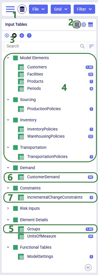
This next screenshot shows the customer and facility locations on a map:

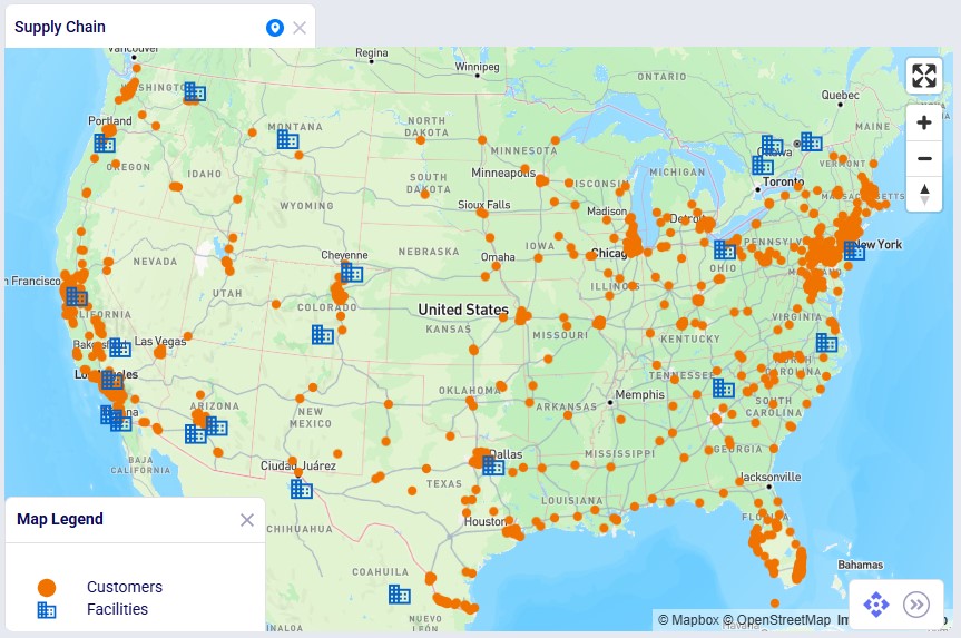
As mentioned, the demand varies quite a lot by period; the following bar chart shows the total demand by period:

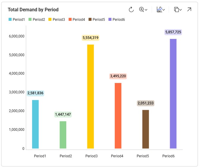
Now, we will take a closer look at the new Incremental Change Constraints input table:

1. We have opened the Incremental Change Constraints input table.
2. In the first column we can choose the Change Type we want to constrain. A drop-down list with the options (Facilities Opened/Closed, Production Increase/Decrease, Lanes Added, Suppliers Added/Removed) is available. In this example model we set up “Production Increase” constraints for all periods, except Period1.
3. Period Name and Period Name Group Behavior – specify the period the constraint applies to. Currently, the Period Name Group Behavior field will always behave like the Enumerate value, regardless of its value. This means the constraint will be applied to each period individually when the Period Name field is set to a group. Here individual records for periods 2-6 have been set up. Note that a group consisting of these 5 periods could have also been used in 1 record instead.
4. Budget and Budget Basis – these specify how much change (the “budget”) is allowed in this period as compared to the previous period for this change type. The basis can be set to either Percentage or Quantity. Here, the budget is set to 10 percent for all records, meaning (for the first record) that the total production in Period2 cannot be more than 10% higher than the total production in Period1. Say the total production in Period1 is 3M units, then the constraint in this first record limits the total production to a maximum of 3.3M units in Period2. If the budget had been set to 100,000 with a Quantity basis, it would mean that the total production in Period2 would be limited to 3.1M units.
5. Like most input tables in Cosmic Frog, this one also has a Status field indicating if a record should be included when the model is run (Status = Include) or not (Status = Exclude). These are often used in scenario items to switch a constraint on or off. Here, all records are set to Exclude, and we will change these to Include in the scenarios where we want to use the Incremental Change feature.

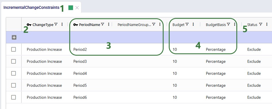
Please note that this table also has a Notes field, which is not shown in the screenshot. Notes fields are also often used by scenarios, for example to filter out a subset of records for which the Status needs to be switched based on the text contained in the Notes field.

Production Smoothing – Scenarios

The following 5 scenarios are included in this example model:

1. In the “1. No Limit Production Fluctuations” scenario no limits are placed on production increases, and we expect production to closely match demand in order to reduce inventory holding costs as much as possible as all other costs will be equal.
2. The “2. Limit Production Fluctuations – 2 Pct” scenario only allows a 2% increase in production from one period to the next. This is achieved through 2 scenario items:
   1. The “Include Incremental change” scenario item switches the Status of all records in the Incremental Change Constraints table to Include.
   2. The “Budget set to 2pct” scenario item sets the Budget field for all records in the Incremental Change Constraints table to 2. Its configuration is shown on the right-hand side in the screenshot.
3. The other 3 scenarios are very similar to the second scenario: they all have the “Include Incremental change” scenario item included to turn on the constraints set up in the Incremental Change Constraints table and each has a scenario item setting the budget field to a different value:
   1. The “3. Limit Production Fluctuations – 5 Pct” scenario limits production increases from one period to the next to 5%.
   2. The “4. Limit Production Fluctuations – 10 Pct” scenario limits production increases from one period to the next to 10%.
   3. The “5. Limit Production Fluctuations – 20 Pct” scenario limits production increases from one period to the next to 20%.

Production Smoothing – Outputs

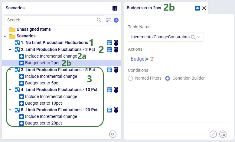
After running all 5 scenarios, we will first look at the 2 new output tables, and then at several graphs set up in the Analytics module specifically for this model.

The following screenshot shows the Optimization Incremental Change Summary output table:

1. For scenarios 2 (max 2% production increase for each subsequent period) and 3 (max 5% production increase), we see from the Actual Change column that for each period the maximum allowed change (the Budget column) for production increase is used.
2. For scenario 4 where a maximum production increase of 10% for each subsequent period is allowed, periods 2, 3, and 6 use all of this budget, whereas periods 4 and 5 do not.
3. For scenario 5 (max 20% production increase), it is the same as for scenario 4: the allowed change budget is entirely used in periods 2, 3, and 6, but not in periods 4 and 5.

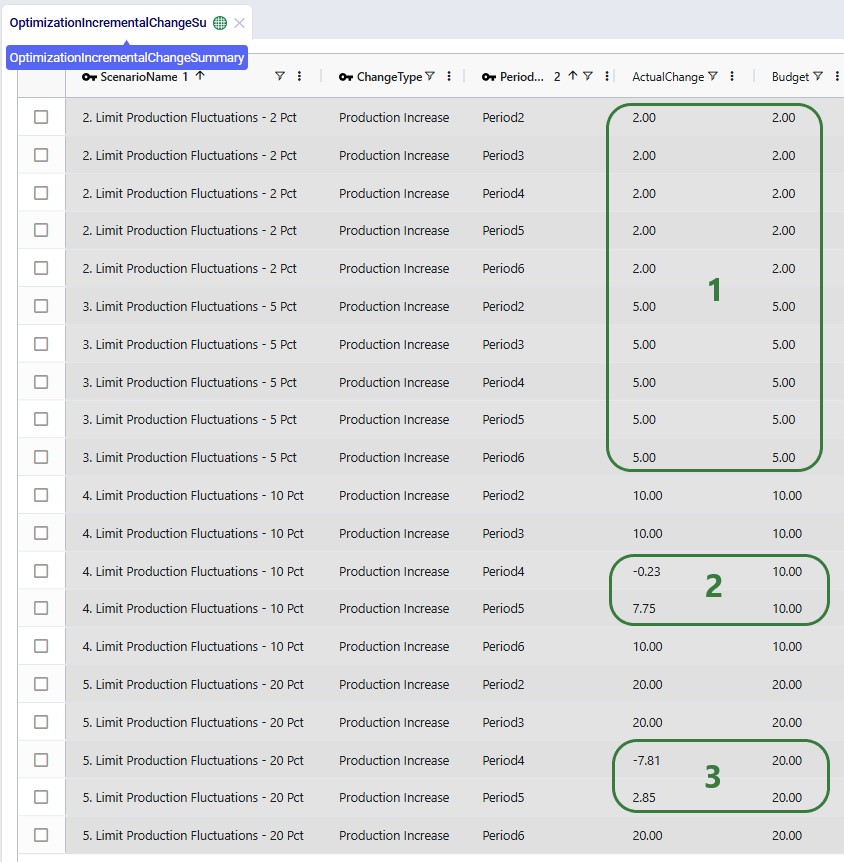
The other new output table, the Optimization Incremental Change Report, contains the changes at a more detailed level. For production increase incremental change types, it indicates the change in production at the individual facilities for the periods the constraint(s) are applied. In the next screenshot, we look at the report which is filtered for the fourth scenario and only the records for Facility_01 are shown:

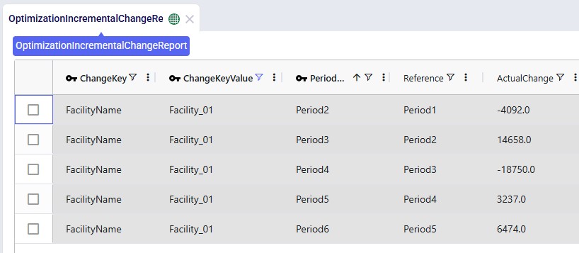
The Actual Change column here reflects the difference in the quantity produced between the period and the referenced (previous) period. The first record tells us that in Period2 Facility_01 produced 4,092 units less than it produced in Period1, etc.

Now, we will look at several graphs set up in the Analytics module. The names of the dashboards containing the graphs start with “Incremental Change - …”. The first one we will look at is the Production by Period graph found on the “Incremental Change – Production by Period” dashboard. Here we compare the first scenario (No Limit) with the most constrained scenario which is the second one (only 2% increase in production allowed in each subsequent month):

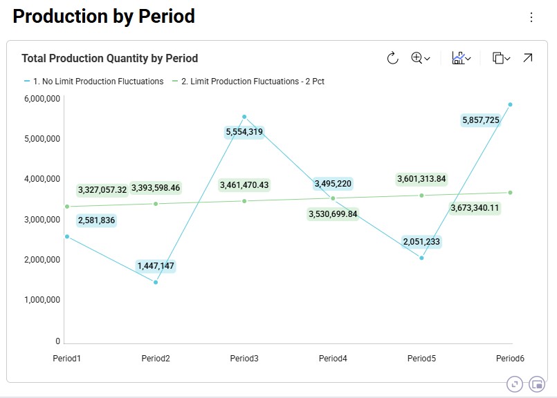
The blue line and numbers represent the production quantities of the first scenario (no limit). Since there are no limits set on how much production can fluctuate, the production is equal to the demand in that period to avoid any pre-build inventory and its holding costs. Since the demand varies greatly between each period, so does the production. For example, in Period2 the quantity produced is 1.45M units and in Period3 this is 5.55M units, which is a 280% increase.

The green line and numbers represent the production quantities of the second scenario (max 2% production increase). To even out the production and stay within the 2% increase restriction, we see that production in periods 1 and 2 is higher in this scenario as compared to the first one. We can deduce that inventory is being pre-built here in order to be able to fulfill the high demand in Period3. We will show the pre-build inventory levels by period in another upcoming dashboard.

The next graph, from the "Incremental Change - Demand and Production" dashboard, compares the production by period for all 5 scenarios using a bar-chart:

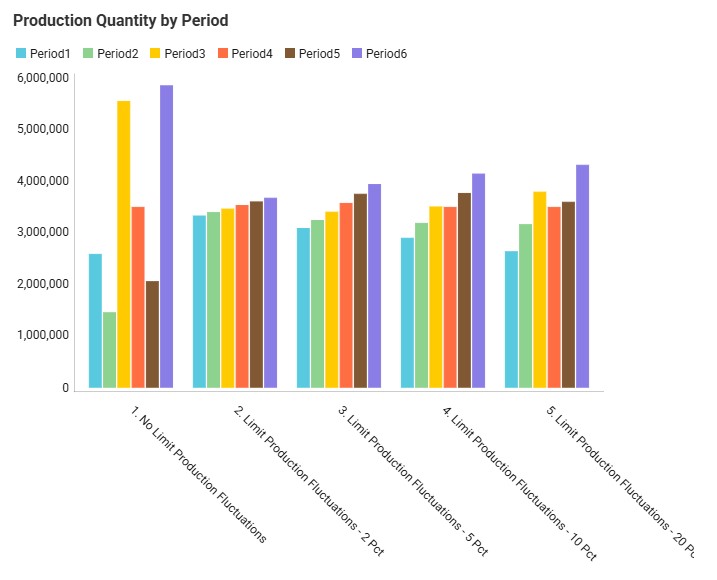
We see the same for scenarios 1 and 2 as we discussed for the previous graph: high fluctuations in scenario 1 and only slight increases period-over-period in scenario 2. Scenarios 3, 4, and 5 gradually allow higher increases in production (5%, 10%, and 20%), and we can see from the production outputs that in order to reduce cost of holding pre-build inventory in stock, the scenarios do show more fluctuations in the production quantity so that product is produced as close as possible in time to when the product is demanded, while adhering to the % increase limitations.

We can also illustrate this by looking at the amount of pre-build inventory across the periods for each scenario, which is shown on the “Incremental Change – Pre-build Inventory” dashboard:

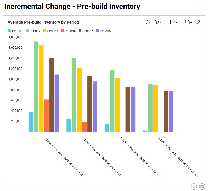
We notice that the first scenario is not shown here as it does not have any pre-build inventory in any of the periods: the production in each period matches the demand in each period to avoid any pre-build holding costs. For the other scenarios, we see, as expected, that the more stringent the limitation on the fluctuation in production quantity is, the more pre-build inventory is being held. In scenarios 4 and 5 (10% and 20% increases allowed), there is no need to have pre-build inventory in Period4 for example, whereas this is needed in scenarios 2 and 3 (2% and 5% increases allowed).

We can of course also look at the costs associated with each of the 5 scenarios, using the Optimization Network Summary output table:

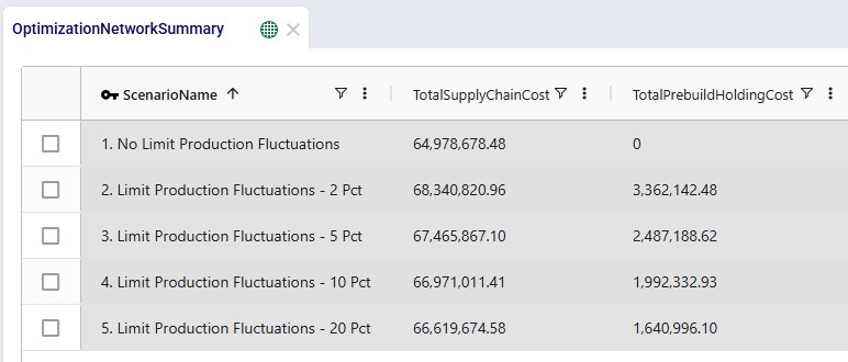
The costs are made up of transportation costs ($41.2M for all scenarios), in transit holding costs ($51k for all scenarios), production costs ($4.2M for all scenarios), outbound handling costs ($19.5M for all scenarios), and pre-build holding costs. Only the pre-build holding costs differ between the scenarios due to the timing of production being different because of the production increase incremental change constraints. As we saw above, no pre-build inventory was held in scenario 1, so the pre-build holding cost for this scenario is 0. Most pre-build inventory was held in the most stringent scenario, scenario #2, and therefore the pre-build holding costs are highest for this scenario, decreasing as the production increase change constraint is gradually loosened from 2 to 20%.

Finally, we will have a look at a map to see the flows from the facilities to the customers:

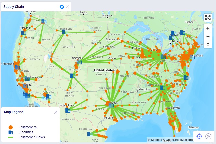
In this map we see all flows for all periods for scenario 3. We notice that customers source from their closest facility. Since this is a multi-period model, we can also configure the map to see the flows for just a single period or a subset of the periods, by using the fold-out periods toolbar located at the bottom-right in the screenshot.

Example Model 2 – Supplier Base Transition

This example demonstrates how Incremental Change can be used to determine the optimal sequence of supplier changes when transitioning from a mixed supplier base to a single-region sourcing strategy.

The model evaluates two potential transitions:

• Moving to all China suppliers
• Moving to all Europe suppliers

Supplier onboarding is limited to two suppliers per quarter, reflecting operational onboarding limits.

In addition, the model evaluates whether adding a new West Coast port and factory improves the network. These locations could realistically only become operational starting in 2028, which is modeled using incremental change constraints.

This example model, "Incremental Change - Supplier Base Transition", can be copied from the Resource Library if you want to follow along.

Supplier Base Transition - Inputs

Model Background

This example is based on the Global Supply Chain Strategy model from the Resource Library (here) and has been modified to demonstrate Incremental Change functionality.

Supplier Base

This model includes two supplier regions:

Europe

• 39 suppliers (Spain, France, Belgium, Germany)
• Ship through Rotterdam Port

China

• 31 suppliers
• Ship through Shanghai Port

The current supplier base consists of:

• 6 European suppliers; they supply 1 raw material each
• 3 Chines suppliers; they supply 1 raw material each

The additional suppliers are included in the model but initially inactive.

This screenshot shows the existing and potential suppliers in Europe:

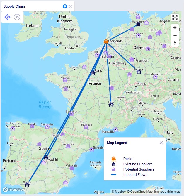
The next screenshot shows the existing and potential suppliers in China:

Network Structure

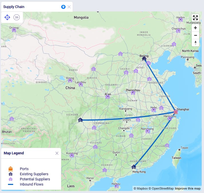
Materials flow through the network as follows:

1. Local Suppliers → Overseas Ports (Raw Materials)
   • Rotterdam (Europe)
   • Shanghai (China)
2. Overseas Ports → North America Ports (Raw Materials)
   • Charleston Port (USA)
   • Altamira Port (Mexico)
3. US / Mexico Ports → Factories (Raw Materials)
   • Princeton Factory (USA)
   • El Bajio Factory (Mexico)
4. Factories → Distribution Centers (Finished Goods)
   • 7 U.S. DCs serving 1,333 customers

The model also includes potential West Coast expansion locations:

• Los Angeles Port
• Reno Factory

These facilities are evaluated in selected scenarios.

The following screenshot shows the port, factory, DC, and customer locations in North America, with the port to factory and factory to DC flows showing too:

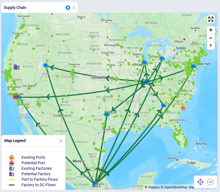
First, we will cover the basic inputs in this model that were added / modified from the original Global Supply Chain Strategy model. After that we will explain the inputs that have been added to model the supplier base transition and those that enable consideration of using the new port and factory on the US west coast.

Basic Model Adjustments

Several changes were made to the base model to support the incremental change example:

Supplier Base Transition

Transition Requirements

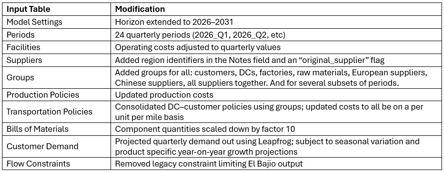
The model evaluates transitions to either an all-Europe or all-China supplier base under the following rules:

• Maximum 2 suppliers added per quarter
• Original suppliers remain fixed during 2026
• Transition occurs during 2027–2029 (12 periods)
• To reduce risk of relying on a single supplier for a raw material (current situation), the final configuration requires:
  • 2 suppliers per raw material, where each supplies at least ~35% of the total
  • 1 raw material per supplier

This supplier base transition is visualized on the following timeline:

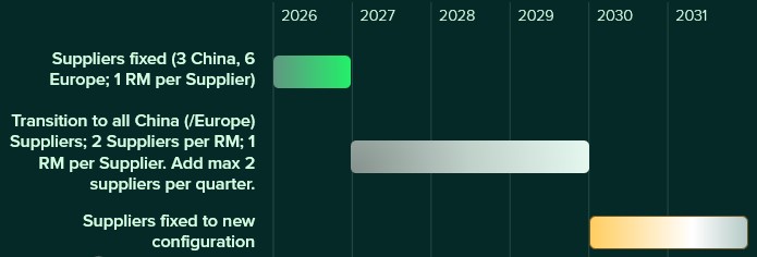
After running scenarios with the above transition settings, we will also run 2 accelerated transition scenarios:

• Maximum 3 suppliers added per quarter
• Transition completed in 6 quarters (Q1 2027 – Q2 2028)

This looks as follows on a timeline:

Supplier Configuration Logic

Supplier Capabilities

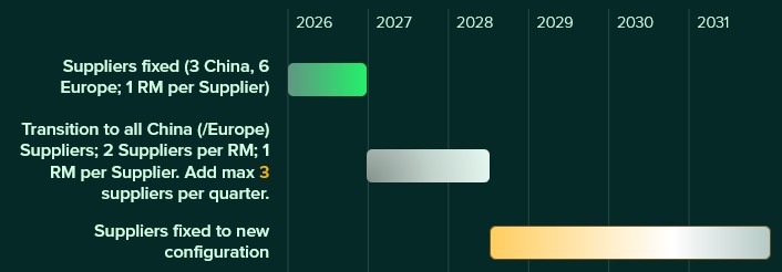
Supplier availability is controlled using two input tables:

Supplier Capabilities

• Defines which suppliers can supply which raw material – each supplier generally is able to supply 2 different raw materials
• Specifies supply costs – on average the unit cost from Chinese suppliers is 25% less than from European suppliers

Supplier Capabilities Multi-Time Period

• Controls when supplier relationships are allowed

Three configuration sets are included:

Scenarios activate the appropriate configuration by switching the Status field to Include for the relevant records.

In the following screenshot of the Supplier Capabilities table, we see 12 (of the 21) suppliers that can supply RM4. Since the Paris supplier is the one which currently supplies this raw material, we see that the Status for that record is set to Include, whereas it is set to Exclude for all others. This is similarly set up for the other 8 raw materials. In scenarios where the supplier base is being shifted, the Status of the other records is set to Include.

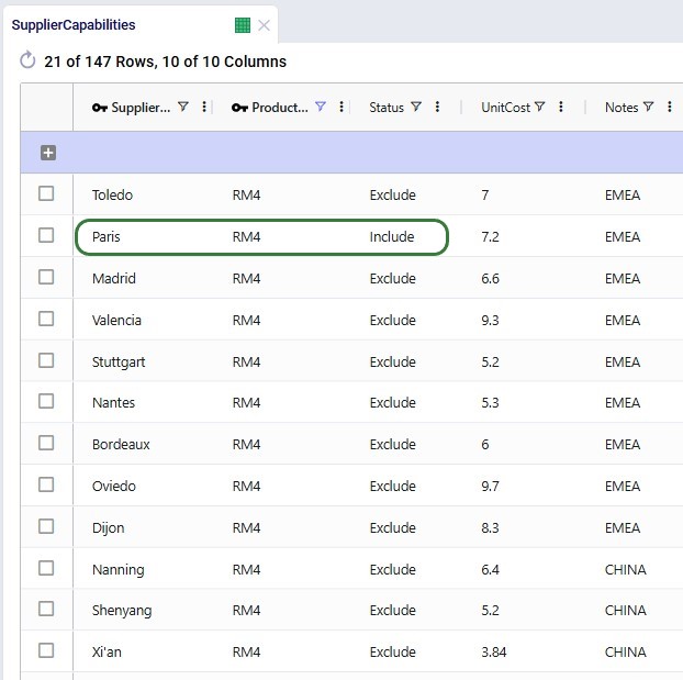
The next screenshot shows the Supplier Capabilities Multi-Time Period table which is filtered for Supplier Name = Chengdu or Mainz and Product Name = RM3. Chengdu (China) is the original supplier for RM3, while Mainz (Europe) is not currently used at all and will be considered for supplying RM3 in scenarios that transition the supplier base to Europe:

1. The first set of records is to be used in scenarios where the currently used 9 suppliers should continue to be used as is. This set of records contains “Baseline” in the Notes field. The total set consists of 9 records, 1 for each RM and its current supplier, where Policy Status = Include indicates they can be used once the record is included (i.e., Status switched to Include) during the whole model horizon (Period Name is set to the “All Periods” group).
2. The second set of records has “China Only” in its Notes field and this set is used in scenarios where we want to transition the whole supplier base to China.
   • For Chengdu – RM3 (the first 2 “China Only” records), we see that once the Status is switched to “Include”, these records indicate that this supplier – RM combination can be used throughout the model horizon since the Policy Status of both these records is set to Include. Since this is the original supplier for RM3, it needs to be able to be used in 2026 (periods 1-4). And, because it is a Chinese supplier, we also want to consider it to be used in periods 5-24 (2027-2031).
   • For Mainz – RM3 (3^rd and 4^th “China Only” records), we see that its Policy Status for both records is set to Exclude. This is because we only want to use the original suppliers during periods 1-4 (2026), which Mainz is not one of and because we are transitioning to only Chinese suppliers and Mainz is in Europe.
3. The third set of records has “Europe Only” in its Notes field and this set is used (its Status switched to Include) in scenarios where we want to transition the whole supplier base to Europe.
   • For Chengdu – RM3 (first 3 “Europe Only” records), we see that once the Status is switched to “Include”, the first 2 of these records have Policy Status = Include. These specify that this supplier – RM combination can be used during the initial fixed supplier phase since it is the current supplier for RM3 (first record for periods 1-4) and also during the transition period (periods 5-16, 2027-2029) as we do not know ahead of time exactly when this supplier will be phased out. The third of these records for periods 17-24 (2030-2031) has Policy Status = Exclude, which means that during this new fixed supplier period it cannot be used. This is because we are moving to an all European supplier base and this is a Chinese supplier.
   • For Mainz – RM3 (4^th and 5^th “Europe Only” records), we see that its Policy Status for the first record is set to Exclude, since it is not the original supplier of this RM. Then for the remaining periods (5-24, 2027-2031) its Policy Status is set to Include. Because it is a European supplier, we want it to be considered during the transition phase (periods 5-16, 2027 - 2029) and should it be selected it needs to be able to be used during periods 17-24 (2030 – 2031) too.

Risk Mitigation Constraints

Minimum Supplier Utilization

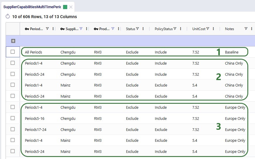
To ensure meaningful dual sourcing, each raw material must be supplied by two suppliers.

To prevent trivial allocations (e.g., one supplier providing only a few units), conditional minimum flow constraints require that each active supplier provides approximately 35% of total supply. This ensures both suppliers meaningfully contribute to supply.

The 2 screenshots below show the setup for RM6 on the Flow Constraints input table:

• Constraint Type = Conditional Minimum means that the flow on the specific lane should either be 0 or otherwise be at least the value set in the Constraint Value field
• Groups are used for the Origin Name and Period Name fields with their associated Group Name Behavior fields set to Enumerate – these constraints will therefore be expanded into all individual origin – period combinations at runtime and be applied each quarter to each supplier – port lane.

Supplier Structure Constraints

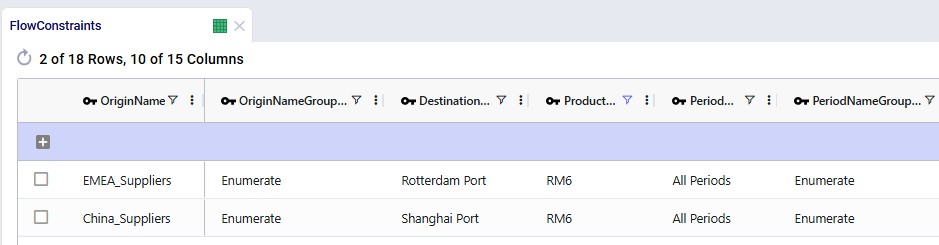
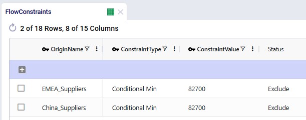
Additional flow count constraints enforce the supplier structure:

• Maximum 3 suppliers per raw material across the entire horizon – the original supplier and the final 2 suppliers
• Maximum 1 raw material per supplier
• Maximum 2 suppliers per raw material during transition
• Final configuration must include two suppliers from the selected region only

These 2 screenshots show the flow count constraints which are used (Status switched from Exclude to Include) in the scenarios where the supplier base is shifted; they are explained underneath the second screenshot:

1. This constraint is used in all scenarios where the supplier base is shifted and ensures that during the whole model horizon (2026 – 2031) each raw material is not supplied by more than 3 suppliers: its original supplier and the 2 in the final supplier base configuration.
2. These 2 constraints are also included in all scenarios where the supplier base is shifted, and they ensure that each supplier does not supply more than 1 raw material.
3. This constraint is also used in all scenarios where the supplier base is shifted; it limits the number of suppliers for each RM to 2 during the transition period. Because the constraint is for the transition period, it is over all suppliers together, since it can be a mix of Chinese and European suppliers during this timeframe.
4. These 2 constraints are included in scenarios where the supplier base is shifted to Europe. They ensure there are 2 European and 0 Chinese suppliers for each RM during the phase of the model where the supplier base is fixed to the new configuration (periods 17-24, 2030 – 2031).
5. These 2 constraints are included in scenarios where the supplier base is shifted to China. They ensure there are 2 Chines and 0 European suppliers for each RM during the phase of the model where the supplier base is fixed to the new configuration (periods 17-24, 2030 – 2031).

Incremental Change Constraints

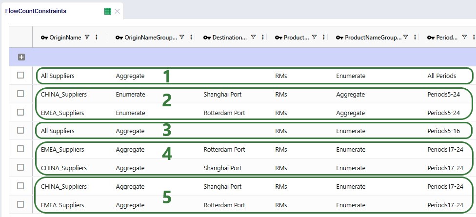
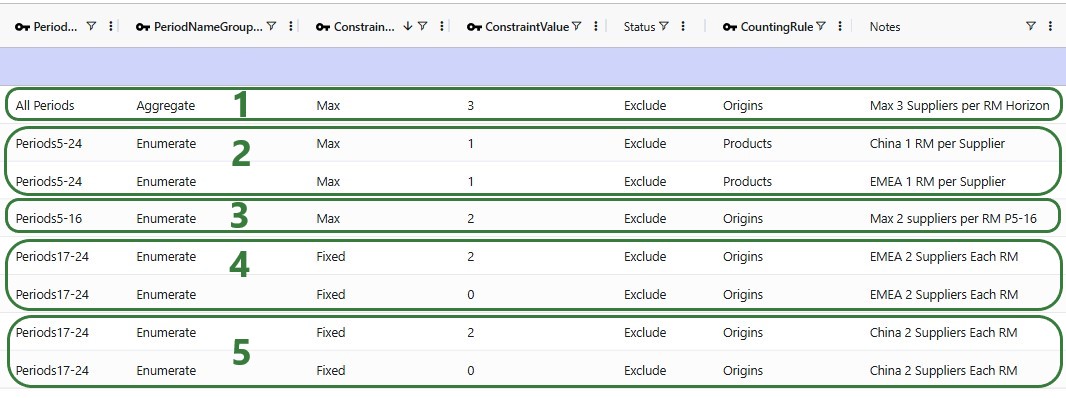
Incremental Change controls the rate of supplier onboarding.

Two configurations are included:

Additional constraints prevent supplier changes after the transition period.

The first 2 constraints shown in the screenshot below are for the standard transition type (Budget = 2 during transition, 0 after) and are included (Status switched to Include) in the scenarios where the supplier base is shifted. The bottom 2 constraints are used together with the one in the second record for scenarios modeling the accelerated transition (Budget =3 during transition, 0 after):

West Coast Expansion Modeling

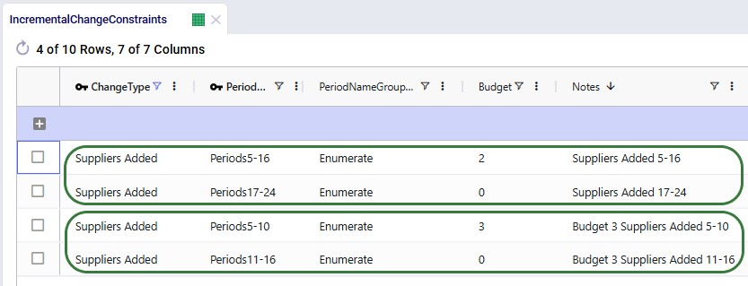
The model evaluates adding:

1. Los Angeles Port
2. Reno Factory

These facilities:

• Are initially set as Potential
• Can only be opened starting 2028
• Are controlled through incremental facility opened change constraints

Facilities table:

Records were added for Los Angeles Port and Reno Factory. As these are currently not existing locations and will be considered for inclusion, their Facility Status = Consider and Initial State = Potential:

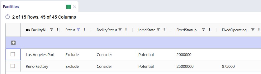
Facilities Multi-Time Period table:

Since we only want to consider including the west coast locations from 2028 onwards, we need to make sure that at the beginning of the model horizon they are closed. This is done by adding 2 records for 2026_Q1 to the Facilities Multi-Time Period table setting the Status for both the Reno Factory and the Los Angeles Port to Closed, see screenshot below. For the remaining periods in the model the Incremental Change Constraints (see further below in this section) take care of when the factory and port are considered for opening.

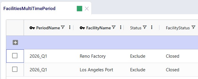
Production Policies table:

Records are added for the Reno Factory so it can manufacture all 3 finished goods, using the existing BOMs:

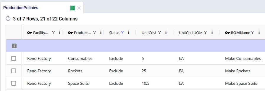
Transportation Policies table:

Records are added so that Los Angeles Port can receive raw materials from the ports in Rotterdam and Shanghai, the Los Angeles Port can ship these to the factory in Reno, and Reno Factory can serve the finished goods to all 7 DCs:

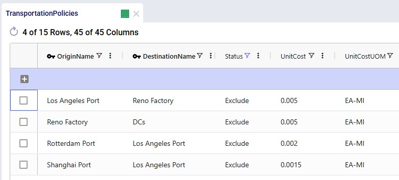
Incremental Change Constraints table:

Here, 2 records are added to set up the desired behavior of allowing the Reno Factory and Los Angeles Port to be added to the network from 2028_Q1 onwards.

• The first record indicates that for periods 2 through 8 (Q2 2026 through Q4 2027) the budget for the Change Type of Facilities Opened is 0. In other words, no facilities can be added to the network during this timeframe.
• The second record specifies that for periods 9 through 24 (Q1 2028 through Q4 2031) the budget for the Change Type of Facilities Opened is 2. This budget is available for each quarter within this period. Since we are only considering adding 2 locations in total (the West Coast port and factory), the budget will only be used in one period or not at all.

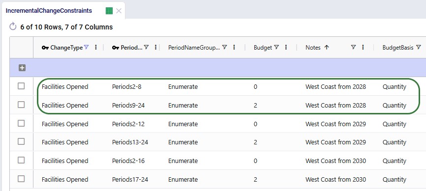
The other 4 "Facilities Opened" records in this table are not used in this model. They were added in case users want to set up and run some scenarios themselves where the west coast port and factory are allowed to be added from 2029 (records 3 and 4) or from 2030 (records 5 and 6) onwards.

Supplier Base Transition – Scenarios

The following table shows the scenarios that were run in this example model. Initially the first 5 were run and based on the results, number 6 and 7 were added and run too:

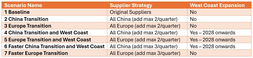
The Scenarios module of this example model looks as follows:

1. For the Baseline scenario, we only need 1 scenario item: the one that sets the Status to Include for the set of Notes = “Baseline” records on the Supplier Capabilities Multi-Time Period table.
2. Scenarios which consider using the west coast port and factory (scenarios 4, 5, and 6) include these 5 scenario items which switch the Status to Include for the records that specify the model elements needed, e.g. including the locations on the Facilities table, including the production and transportation policies, etc. The “Include Reno Considered from 2028 Constraint” scenario item changes the Status of the 2 records with Notes = “Reno from 2028” on the Incremental Change Constraints table to Include.
3. Scenarios which transition the supplier base to China (scenarios 2, 4 and 6) include these 7 scenario items. The scenarios that transition the supplier base to Europe (scenarios 3, 5, and 7) also use 4 of these and they have 3 scenario items that are the Europe-specific version of the other scenario items. The “Include Suppliers Added P5-16 Budget 2 Constraints” scenario item changes the status of the 2 records needed to set the transition period and budget on the Incremental Change Constraints table to Include.
4. If users want to see for themselves what happens when the west coast port and facility are allowed to be used from 2029 or 2030 onwards, instead of from 2028 onwards, they can use these 2 unassigned items to do so. Steps to set up a new scenario using these would for example be: 1) copy the scenario of interest, say scenario 4, 2) remove the “Include Reno Considered from 2028 Constraint” from this scenario, and 3) add 1 of the 2 currently unassigned scenario items to this copied scenario.

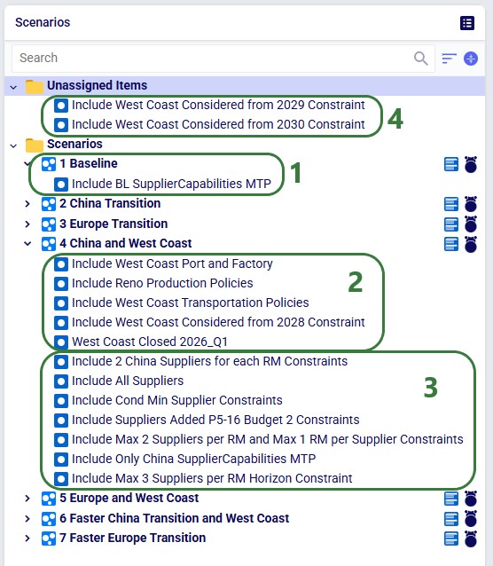
For running the scenarios, 2 of the technology parameters were changed from their defaults:

• The MIP Relative Gap Percentage was reduced to 0.00001 (=0.001%). Due to the large numbers in the model and the relatively small differences between feasible solutions (e.g. the cost difference between phasing a supplier in or out a period earlier or later could be smaller than 0.01% of the total supply chain cost), better solutions were found with this smaller gap, while all scenarios solve in less than 3 minutes.
• The Feasibility tolerance was increased to 0.00001 to avoid incorrect infeasible results.

Supplier Base Transition – Outputs

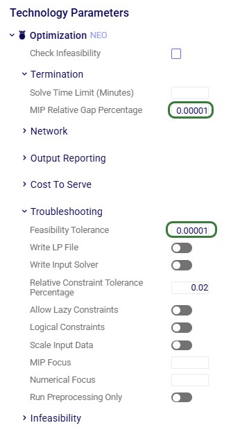
After running all scenarios, it is time to examine the outputs. We will start by looking at the new Optimization Incremental Change Summary and Optimization Incremental Change Report output tables and then visualize the supplier base changes on maps and a timeline grid. For these, we will mostly focus on scenarios 4 and 5 which show all incremental change constructs we have used in the model. Finally, we will also have a look at the financial impact and compare all scenarios.

The Optimization Incremental Change Summary table shows how much of each change budget is used in each period. Two screenshots of this output table are shown next; in both, the table is filtered for scenario number 5 (field not shown) where the supplier base is moved to Europe and adding the west coast locations to the network is considered:

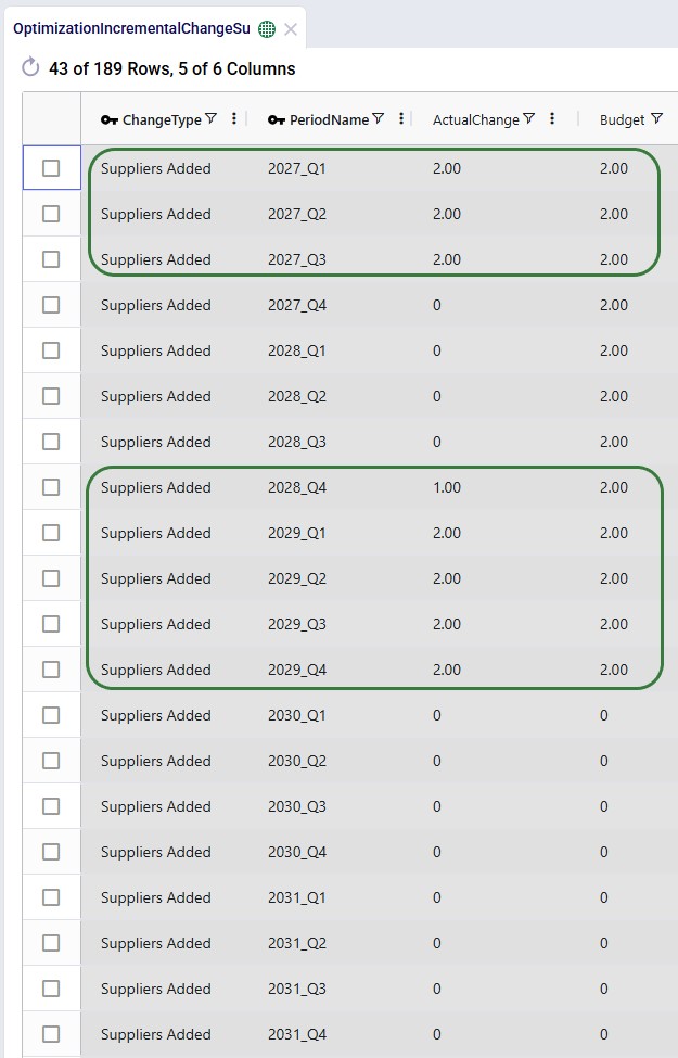
During each of the first 3 quarters of the transition period 2 suppliers were added, then there is a pause in adding suppliers, and towards the end of the transition period, another 9 suppliers are added, essentially as late as possible. We can interpret this as:

1. Several European suppliers are added early because they are the cheapest options for 6 of the RMs. These suppliers are added in the most cost-efficient order possible (i.e., those providing the highest cost savings first).
2. Since the model is not adding 9 new suppliers at this stage, we can hypothesize (and we will check this through other outputs further below) that 3 of the original suppliers keep being used, either to supply the RM they have been supplying until now or a different one.
3. The 9 Remaining suppliers are added towards the end of the transition period to satisfy the two-supplier requirement while minimizing costs.

The next screenshot shows the same table, still filtered for scenario 5, but now the records for the Facilities Opened change type constraints are shown:

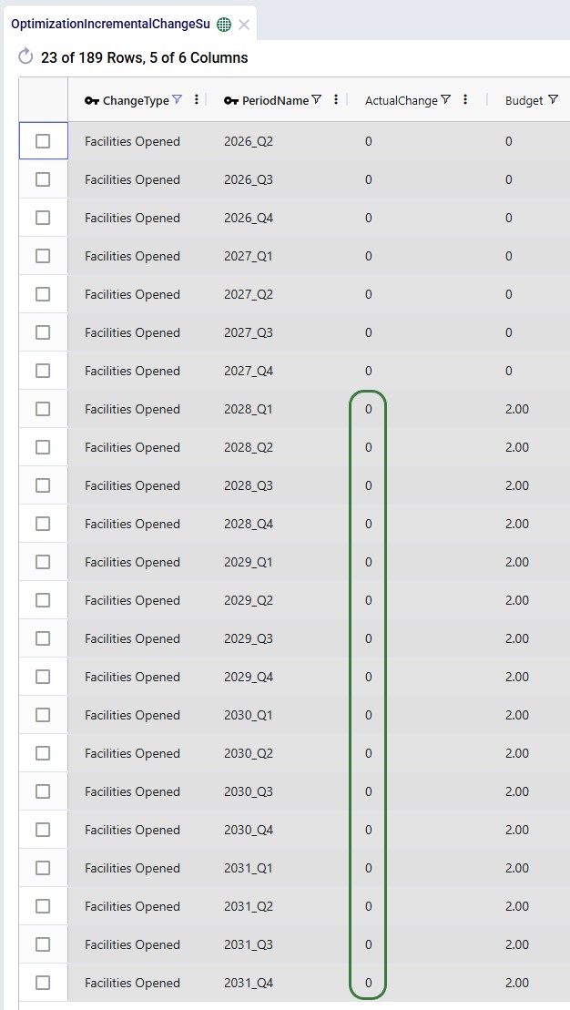
We see that the budget was 2 for each of the periods in the 2028 – 2031 timeframe, but the Actual Change column indicates that no change (0) happened in any of those periods. In this scenario, it is not beneficial to start using the west coast port and factory anytime from Q1 2028 onwards.

Next, we will cover the Optimization Incremental Change Report output table. This table has a record for each incremental change that was made, including details on what the change was. This table is filtered for scenario 4 (field not shown) where the supplier base is moved to China and the west coast locations are considered (note that records beyond Q1 2029 are not shown here):

From the first 4 records for Q1 of 2027, we can tell that suppliers in Hefei and Taiyuan were added to the supplier base, while suppliers in Lyon and Madrid were removed. Similarly, 2 suppliers are added and removed in each of the next 2 quarters. Then in Q1 of 2028, the Reno Factory and Los Angeles Port are opened, which is apparently beneficial to do as early as possible when moving the supplier base to China. This is due to the lower transportation costs because of the shorter distance from Shanghai to Los Angeles as compared to going to the Charleston or Altamira ports.

In summary:

• When transitioning to European suppliers, the model does not open the Los Angeles Port or Reno Factory, indicating the west coast expansion is not cost-effective under this sourcing strategy.
• When transitioning to Chinese suppliers, the model opens the Reno Factory and Los Angeles Port as early as possible, reducing ocean shipping distance and transportation costs.

The next map shows the final configuration of the supplier base for scenario 4 where it is moved entirely to China. Notice that we have used the Period selector bar (at the top of the map) to show the map for Q1 of 2030 when the transition is complete. You can use this period selector to step through the periods to see the gradual changes over time.

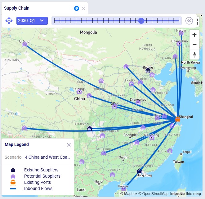
The next map is also for scenario 4 but now showing the North American locations and flows (except for the DC – Customer flows) for the same period of Q1 2030. We see that the Los Angeles Port and Reno Factory are being used in this scenario.

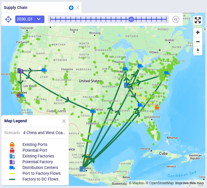
Similar to the first map shown above, the next map shows the final supplier configuration in Q1 2030 for scenario 5, where the whole base is moved to Europe:

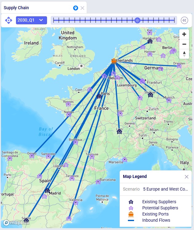
The next 2 timeline grids on the Supplier Transition Timeline dashboard (Analytics module) are generated from a custom table “timeline_rm_bysupplier_byperiod”, which in turn was generated from the Optimization Supply Summary output table. The appendix describes the steps to create the custom table and how to re-create it in case (new) scenarios are added / adjusted and run.

The first screenshot is for scenario 4, the second for scenario 5. They show which supplier supplies which RM when. Note that Q1-Q3 of 2026 are not included as the supplier configuration is equal to the Q4 2026 configuration. Similarly, the timeframe of Q2 2030 through Q4 2031 is not included in this dashboard either, since the supplier configuration is equal to the Q1 2030 configuration. Not all suppliers and period columns are shown in the screenshots, users can scroll horizontally and vertically in the dashboard to examine the full timeline.

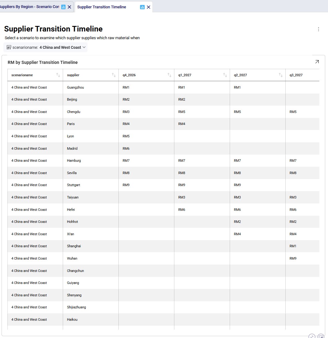
Some things we notice here for scenario 4 are:

1. Guangzhou is the original supplier for RM1 and is phased out from Q3 2027. However, it is also the second-best option to supply RM7, so it is phased back in from Q4 2029.
2. Chengdu is the original supplier for RM3, which it drops as soon as possible, and then switches to supplying RM5.
3. European suppliers Hamburg and Sevilla are being used for RM7 and RM8 for as long as possible, suggesting all China suppliers are more expensive for these 2 RMs.

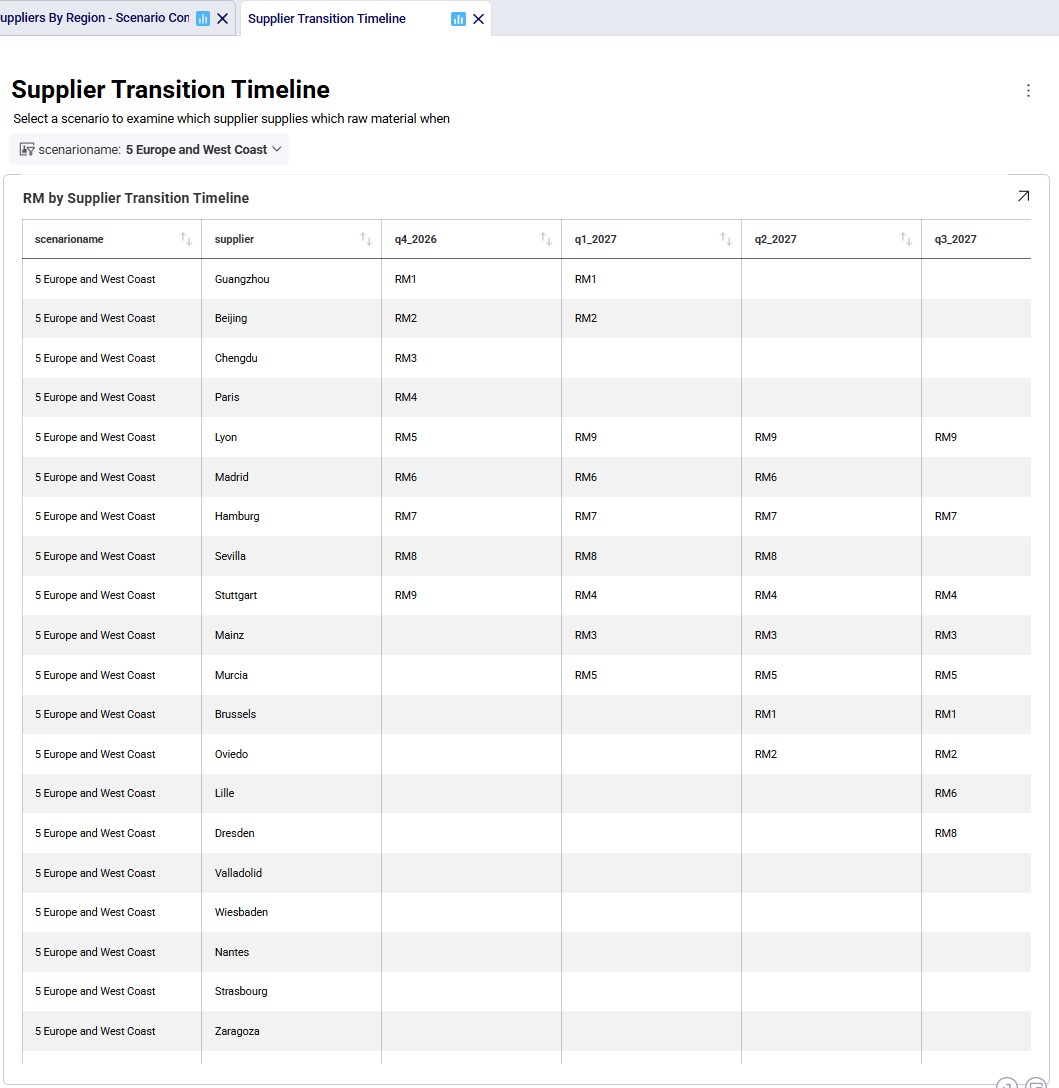
Some things we notice examining the above grid for scenario 5 are:

1. Lyon is the original supplier for RM5, which it drops as soon as possible, and then supplies RM9 for the rest of the model horizon for which it must be the cheapest supplier.
2. Madrid originally supplies RM6, and once Lille comes online it stops supplying it. However, it must still be the second-best option for supplying this raw material as it comes back online supplying RM6 from Q3 2029 onwards. The same thing happens with RM8 at Sevilla.
3. Stuttgart is the original supplier for RM9, which it drops as soon as possible, and then supplies RM4 for the rest of the model horizon for which it must be the cheapest supplier.

Since we are interested in looking at the impact of requiring the supplier base to be transitioned over sooner, scenarios 6 and 7 were run too where the budget for adding suppliers is set to 3 per quarter. We know from scenarios 4 and 5 that the west coast locations are only used when moving the supplier base to China, therefore we run scenario 6 (where we speed up the transition to the China supplier base) with these locations still considered. We do not consider them in scenario 7 where we speed up the transition to the Europe supplier base.

We will now have a look at how the costs compare for all 7 scenarios that were run with the next 2 screenshots of the Optimization Network Summary output table and the screenshot of the “Financials: Scenario Cost Comparison” chart. The latter can be found on the Scenario Comparison dashboard in the Analytics module:

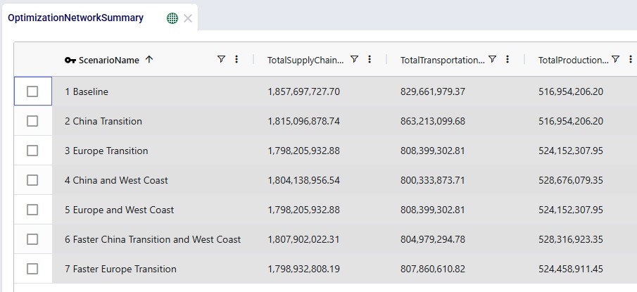
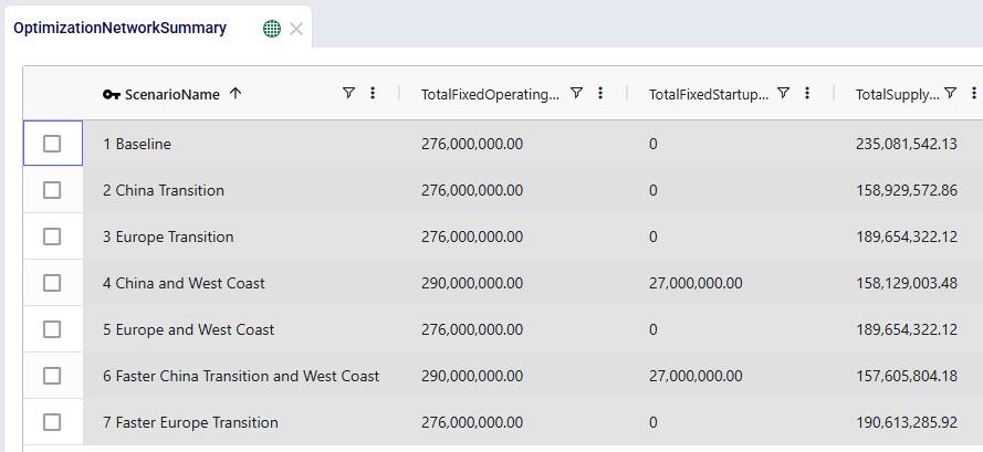
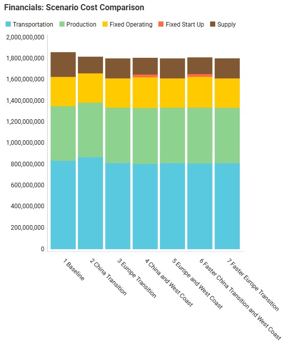
Comparing all scenarios reveals:

1. The baseline configuration is the most expensive.
   1. It is the overall most expensive scenario by more than $40M (over 6 years) as compared to the other 6 scenarios, which are all relatively close to each other when looking at the total supply chain cost.
2. Transitioning to European suppliers provides the lowest overall cost.
   1. Scenarios 2 and 3 where the supplier base is transitioned entirely to China and Europe, respectively, both show considerable cost savings as compared to the baseline. This reduction mostly comes from the lower supply costs, even outweighing the increased transportation costs of scenario 2 (more expensive ocean shipping from Shanghai as compared to from Rotterdam). In scenario 3 it is interesting to see that the production costs increase as compared to the baseline, but these are more than offset by the reduction in transportation costs: the European suppliers ship more to Charleston Port than Altamira Port (reducing the transportation costs as they are distance based), which leads to producing more at the Princeton factory where it is on average more expensive to produce than at the El Bajio Factory. Based on these 2 scenarios, moving the supplier base to Europe makes the most sense financially, since it would be nearly $17M cheaper than moving the supplier base to China.
3. Transitioning to Chinese suppliers becomes more competitive when the West Coast expansion is included.
   1. For scenarios 4 and 5, which are the same as 2 and 3 but with the added option of starting to use the west coast port and factory, we see that scenario 5 has the exact same outputs as scenario 3. This is because it is not cost effective to open the US west coast locations when shifting the supplier base entirely to Europe, and therefore scenarios 3 and 5 have the same outcome. For scenario 4, we do see that using the Los Angeles Port and Reno Factory from 2028 onwards is beneficial: the overall cost of this scenario is about $11M less than for scenario 2. These savings are due to a big reduction in transportation costs ($63M) by going from China to the US west coast and a smaller reduction in supply costs (around $1M), which together outweigh the increases in production, fixed operating, and fixed startup costs (combined around $53M). Even though the total costs for the supplier base transitioning to China has come down in scenario 4 as compared to scenario 2 by using the west coast locations, the total cost is still about $6M higher as compared to transitioning to a European supplier base (scenario 3).
4. Accelerated transition to Europe increases cost slightly but could be operationally desirable.
   1. With the knowledge from the previous 5 scenarios, we decided to run 2 more scenarios, scenarios 6 and 7. Scenario 6 still transitions the entire supplier base to China and allows the west coast locations to be used from 2028. However, the supplier base transition now needs to be completed faster within 1.5 years. Similarly, scenario 7 still shifts the entire supplier base to Europe, but also at a faster pace, and does not consider using the west coast locations. We see that requiring a quicker transition adds costs to both scenarios, but more to scenario 6 than to scenario 7 (close to $4M scenario 6 vs 4, and a little under $1M scenario 7 vs 5). The relatively low additional cost for a quicker transition to an all-European supplier base may make this option a viable one if it can be achieved operationally.

Finally, the following 4 charts for scenarios 4-7 which show the number of suppliers by region over time can be found in the “Suppliers by Region – Scenario Comparison” dashboard in the Analytics module:

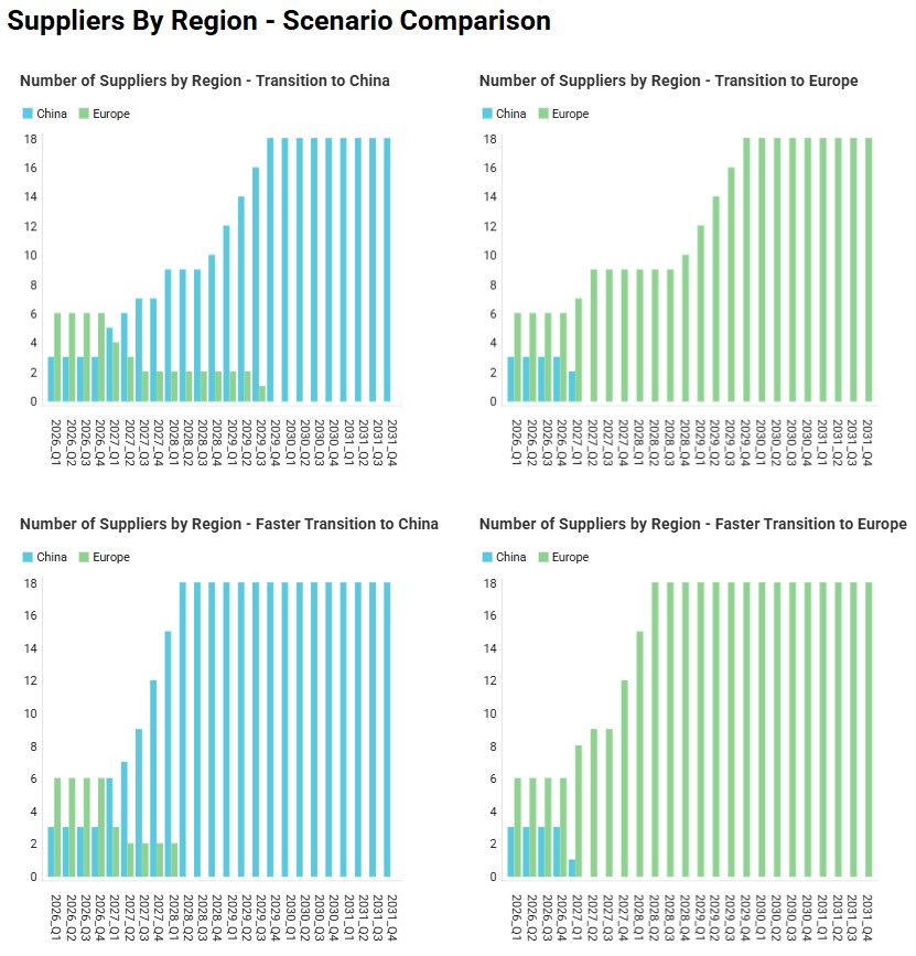
Please do not hesitate to contact Optilogic support at support@optilogic.com in case of questions or feedback.

Appendix –Refreshing the Supplier Transition Timeline Dashboard

To create the timeline grid on the Supplier Transition Timeline dashboard, we first created a custom table named timeline_rm_bysupplier_byperiod, where we added columns for scenarioname, supplier, and 1 column for each period in the model. The latter we named q1_2026, q2_2026, etc. rather than 2026_Q1, 2026_Q2, etc. (which is how the periods in the model are named) as column names in custom tables cannot start with a digit.

Next, this table was populated from the outputs in the Optimization Supply Summary output table, using a SQL Query, which is saved in the model and can be used to refresh the custom table if scenarios are modified/added and (re-)run. For this we use the SQL Editor application on the Optilogic platform:

1. The SQL Editor application can be opened by clicking on its icon in the list of applications on the left-hand side while logged into the Optilogic platform. Should you not see the icon for the SQL Editor, then click on the icon with 3 horizontal dots to see more applications in the list.
2. Select the model, here Incremental Change – Supplier Base Transition, from the drop-down if it is not yet selected here.

The following screenshot shows the central part and right-hand side panel of the SQL Editor application:

1. In the panel on the right-hand side click on the second icon to show the list of bookmarked queries.
2. There is one bookmarked query in this model’s database; to edit or open it, we can click on the pencil icon.
3. The SQL code of the query is now shown in the central part of the SQL Editor (not all is shown in the screenshot).
4. To remove previous outputs from the custom timeline_rm_bysupplier_byperiod table and re-populate it with the latest outputs in the Optimization Supply Summary output table, click on the Execute Query button. Now the table and the Supplier Transition Timeline dashboard that uses it as input will be updated.

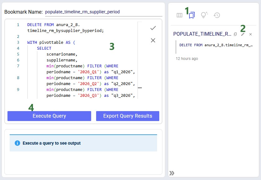
Please note that this custom table, the Supplier Transition Timeline dashboard, and SQL Query to populate it are specific to how this model is set up. All three will need to be updated if the model is changed in certain ways. For example, when adding/removing/renaming periods or if it becomes possible for 1 supplier to supply more than 1 raw material within a period.

Scenarios let you rapidly explore "what-if" questions against an existing Cosmic Frog model. Define one or more data changes (scenario items), run the scenarios, then compare outputs - all without altering your baseline input data.

Quick Start

Follow these five steps to run your first scenario:

1. Open the Scenarios module from the Module menu (top left).
2. Select an existing scenario (e.g., Baseline) or create a new one via right-click → New Scenario.
3. Add a scenario item: right-click the scenario → New Item. Choose a table, specify a column change in the Actions field, and optionally apply a filter.
4. Click the green Run button (top right) and configure technology parameters.
5. Analyze results in the output tables or charts - compare across scenarios side by side.

💡 Tip: Use Leapfrog (Cosmic Frog's AI assistant) to create scenarios and items from plain-language prompts - no manual configuration needed.

What Is a Scenario?

A scenario defines one or more input-table changes to apply before running a solve. Common examples include:

1. Adding candidate locations to evaluate for network expansion
2. Adjusting demand quantities by a percentage for a customer or product subset
3. Modifying transportation or facility costs
4. Switching a set of customers / products between Include and Exclude status
5. Adding or removing limitations on flow, production, and inventory

In the context of this documentation, we mean the following with scenario and scenario item:

• Scenario: a runnable set of inputs based on the data in the input tables, modified with a set of changes (1 or multiple scenario items)
• Scenario item: makes a specific change to all records or a subset of the records in an input table

In other words: a scenario without any scenario items uses all the data in the input tables as is (often called Baseline); most scenarios will contain 1 or more scenario items to test certain changes as compared to a baseline.

The Scenarios Module

Open the Scenarios module from the Module menu. A freshly opened module looks like this:

1. Click the Module menu and select Scenarios.
2. The Unassigned Items folder holds scenario items not used by any scenario.
3. The Scenarios folder lists all scenarios. Expand or collapse it with the caret icon.
4. A Baseline scenario is created by default.
5. The icon to the right of each scenario shows its engine (technology). Use the Technology filter at the top to show only scenarios for (a) specific engine(s).

Scenario Drop-Down Menu

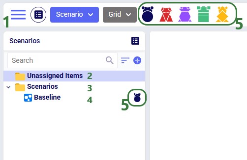
The Scenario drop-down (top of module) provides quick access to common actions:

1. Click on the Scenario drop-down menu to open it.
2. New Scenario - creates a new scenario without any scenario items.
3. New Item - creates a new scenario item in the currently selected scenario.
4. Duplicate - makes a copy of the currently selected scenario or currently selected scenario item:
   1. Scenario - the whole scenario is copied into a new scenario which can be named by the user or otherwise the name will be the original postfixed with (1), (2), etc. The copy contains all the same scenario items as the original.
   2. Scenario item - a copy of the scenario item is added to the current scenario. The copy can be named by the user or otherwise will have the original name postfixed with (1), (2), etc.
5. Rename - edit the name of the currently selected scenario or scenario item. When renaming a scenario that contains outputs, these outputs will be deleted.
6. Copy Name - copies the name of the currently selected scenario or scenario item to the clipboard.
7. Delete - removes the currently selected scenario(s) and/or scenario item(s). A confirmation message will come up prior to the actual removal. See also the Deleting Scenarios and Items section further down.
8. Delete Scenario Results - removes the results of the selected scenario(s) from all output tables, see also the Deleting Scenario Results section further down.

Switching a Scenario's Technology

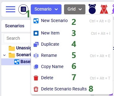
Each scenario is associated with one engine. To change it, select the scenario and use the radio buttons in the central panel:

1. Click the scenario to select it.
2. In the central panel, select a different technology using the radio buttons.

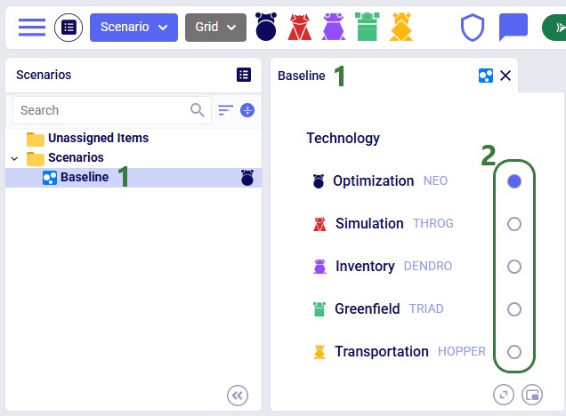
📝 Note: Running with multiple technologies

You can solve the same scenario with more than one engine sequentially: assign the first technology → run → change technology → run again. Be aware that any scenario edits between runs may cause results to differ for subsequent runs.

💡 Tip: Dendro workflow

To optimize inventory policies with Dendro: first build and validate a Throg (simulation) scenario, then switch its technology to Dendro and run.

Creating Scenarios and Items

Creating a New Scenario

Right-click an existing scenario or the Scenarios folder and choose New Scenario, or use the New Scenario option from the Scenario drop-down menu. Enter a name when prompted:

Creating a Scenario Item

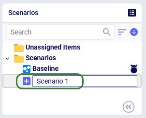
Select the target scenario, then right-click → New Item (or use the Scenario drop-down). Name the item - its configuration panel opens automatically:

1. The new item's configuration opens in the central panel.
2. Select the input table to modify from the Table Name drop-down.
3. A Search box can be used to filter the table list; the Sort icon toggles alphabetical order.
4. We select the Customers table.

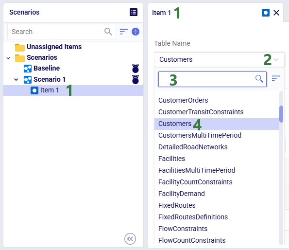
After selecting the table, specify the change in the Actions field. Intelli-type suggests column names as you type:

1. Start typing a column name - intelli-type shows matching columns.
2. Use arrow keys to navigate and Tab to autocomplete.

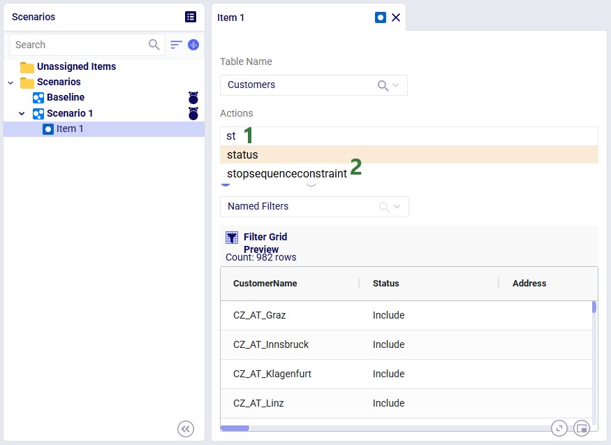
Once the column to change has been typed in, we can set its new value. In our example we want to set the value of the status column to Exclude:

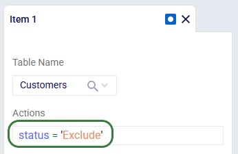
Intelli-type also validates syntax. Incorrect quote style (need to use single quotes, not double quotes):

Unrecognized column name:

📝 Note: For full Actions syntax, see the Writing Syntax for Actions Help Center article.

Filtering Which Records a Scenario Item Affects

By default, a scenario item's action applies to every record in the selected table. Add a filter to restrict which records are changed. Two methods are available:

Named Filters (Recommended)

If Named Filters exist for the selected table, you can apply one directly to the scenario item:

1. In the Conditions area, select Named Filters.
2. Open the Named Filters drop-down to see available filters for the table.
3. Use the Search box to filter the list of filters.
4. Use the Sort icon to change the order of the filters, options are:
   1. Default: sorted in the order they were added to the table.
   2. Name: sorted in (reverse) alphabetical order.
5. Check a filter to apply it. Only records matching that filter will be changed by the Actions field.

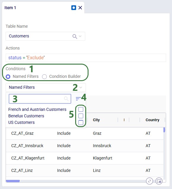
After selecting a filter, the Filter Grid Preview updates to show exactly which records will be affected:

1. The active filter name, "US Customers" here, appears at the top right of the preview. Click x to remove it; hover over it to bring up a tooltip with the entire filter name.
2. The row count shows how many records match - and will be updated.
3. The preview grid confirms the filtered subset (e.g., only US customers).

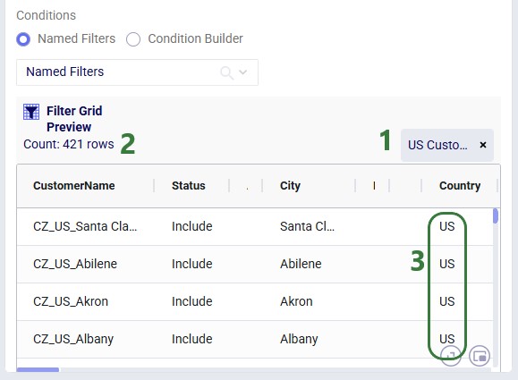
💡 Tip: Why prefer Named Filters?

Named Filters are pre-validated - you have already confirmed they select the right records when creating the filter. The Condition Builder requires you to write syntax manually, which is more error-prone. Named Filters also show a record preview. (Preview for Condition Builder is coming soon.)

📝 Note: One Named Filter per scenario item

Each scenario item supports a maximum of one Named Filter. If you need to combine multiple filter conditions, create a new Named Filter that merges all required conditions.

Condition Builder

Use the Condition Builder when no applicable Named Filter exists, or for ad hoc conditions:

1. Select Condition Builder in the Conditions area.
2. Type the condition expression. Intelli-type column-name suggestions are available here too.

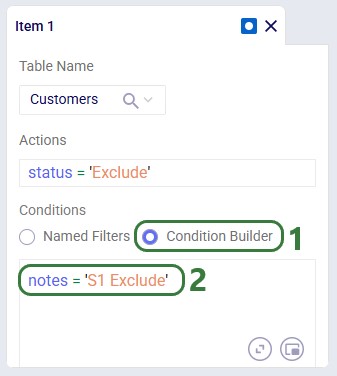
📝 Note: For condition syntax, see the Writing Syntax for Conditions Help Center article.

Scenario Item Execution Order

When multiple items modify the same column in the same table, they execute top-to-bottom. Order matters. Consider the following 2 scenarios where both scenario items are applied to the Quantity column in the Customer Demand table:

1. This scenario contains 2 items: first the demand quantity is multiplied by 2 and then 10 units are added. If the original demand quantity is 100, this scenario changes it to: 2*100 + 10 = 210.
2. This scenario contains the same 2 items but in reverse order: first 10 units are added to the demand and then it is multiplied by 2. For original demand quantity of 100, this results in: (100+10) * 2 = 220.

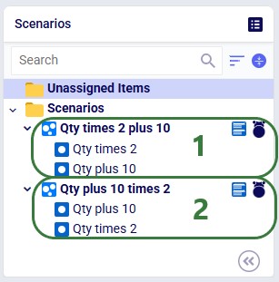
💡 Tip: Drag items up or down within a scenario to reorder them.

Item Assignments

A single scenario item can be shared across multiple scenarios. The Item Assignments panel (right side) appears automatically when an item is selected:

1. The selected item's configuration appears on the left.
2. The Item Assignments panel on the right lists all scenarios.
3. Use the Search box to filter the scenario list.
4. Use the top checkbox to select/deselect all scenarios at once.
5. Check or uncheck individual scenarios to add or remove the item.
6. The counts at the bottom show total scenarios (18 here), how many use this item (Selected: 12 here), and, when filtered by the Search box, how many are currently filtered.
7. Collapse the panel using the >> icon.

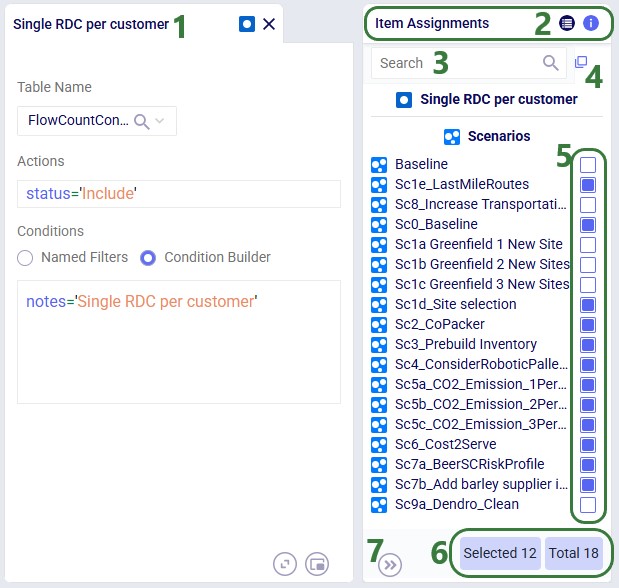
Switch to the Item Information tab on the same panel to edit the item's name or add a description:

1. Click on the second item of the 2 at the top of the pane to switch to the Item Information tab.
2. The Item Name is shown and can be edited if required.
3. Add a description for complex items or collaborative workflows - it appears alongside the item name.
4. Drag the corner of the description box to resize it.

Scenario Assignments

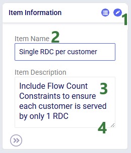
The Scenario Assignments panel (right side) appears when a scenario is selected, showing all available items and which are assigned:

1. The selected scenario's technology assignment is shown on the left.
2. The Scenario Assignments panel on the right lists all items.
3. Use the Search box to filter the item list.
4. Use the top checkbox for bulk selection/deselection.
5. Check or uncheck individual items to add or remove it.
6. The counts at the bottom show total items (8 here), how many are assigned (Selected: 3 here), and, when filtered by the Search box, how many are filtered.
7. Collapse the panel using the >> icon.

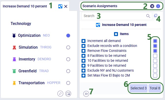
Switch to the Scenario Information tab to edit the scenario name or add a description:

1. Click on the second item of the 2 at the top of the pane to switch to the Scenario Information tab.
2. The Scenario Name is shown and can be edited if required.
3. A Scenario Description can be added here; especially useful for complex scenarios and/or when working collaboratively.
4. Drag the corner of the description box to resize it.

Scenario List Features

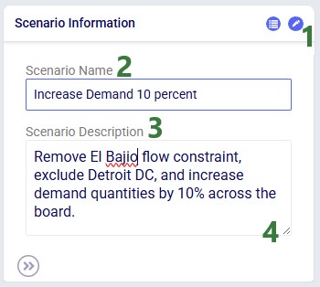
The scenarios list includes several navigation and status indicators that become useful as your model grows:

1. Use the Search box to quickly filter the list down to any scenarios and items containing the search text.
2. The Sort icon enables sorting the scenarios list in the order they were added ("Default") or alphabetically ("Name"). Choosing the same option again reverses the sort order.
3. Click on the Collapse/Expand All icon to either collapse all scenarios and the Unassigned Items folder or to expand them.
4. Users may initially set up scenario items which later on are no longer used by any of the scenarios. These are then shown in the Unassigned Items list. These can be deleted. However, they can also be kept if anticipating using them in future scenarios.
5. Use the caret icons to the left of the scenario names to expand/collapse individual scenarios, i.e. show all or none of its items.
6. A scenario can have anywhere from 0 to many scenario items. This one has 4.
7. If scenario results are available in the output tables, a blue report icon is shown to the left of the scenario's technology icon. The next screenshot shows the tooltip that comes up when hovering over this icon:

1. Hover over the blue report icon for the Results Information tooltip to come up.
2. The tooltip shows the engine used and when the run completed.
3. A link opens the relevant output summary table directly:
   • Neo → Optimization Network Summary
   • Hopper → Transportation Summary
   • Triad → Optimization Greenfield Network Summary
   • Throg → Simulation Network Summary Replication Detail
   • Dendro → Simulation Evolutionary Algorithm Summary

Running Scenarios

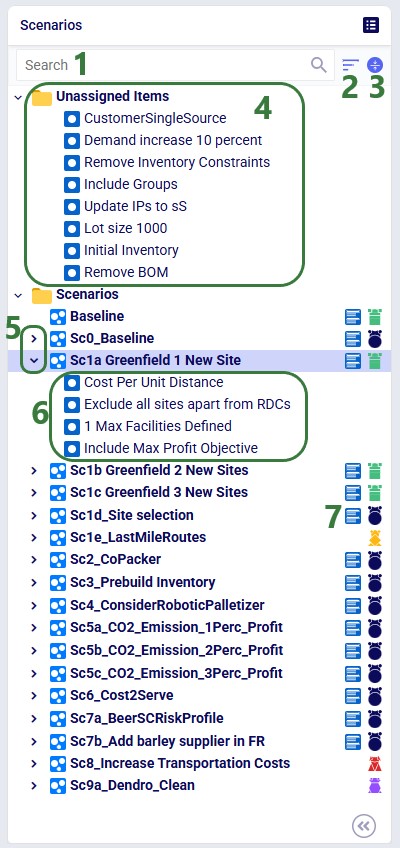
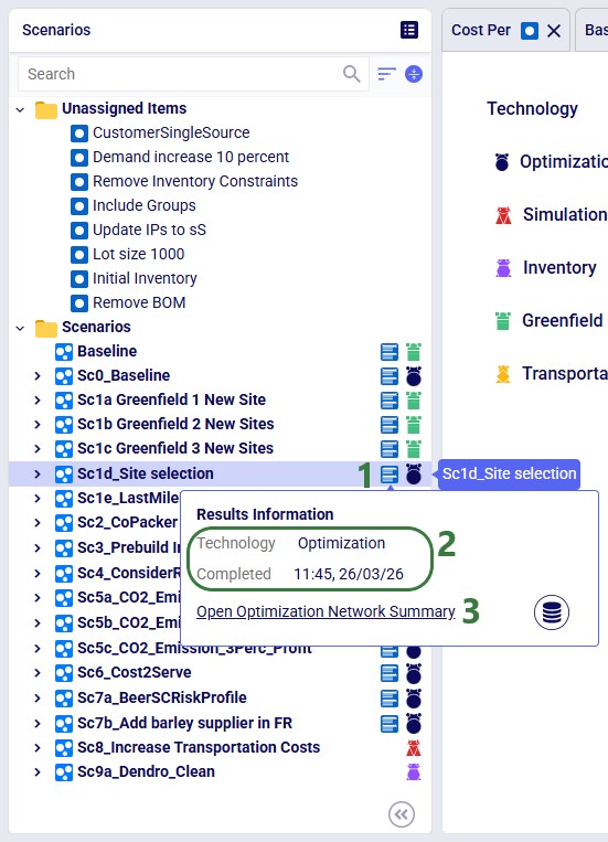
Click the green Run button (top right in Cosmic Frog), select the scenario(s) to solve, and configure technology parameters. See the Running Models & Scenarios in Cosmic Frog Help Center article for full details.

Sensitivity at Scale (S@S) Scenarios

Sensitivity @ Scale automates demand-quantity and transportation-cost sensitivity analysis with a single click. See the Sensitivity at Scale Scenarios Help Center article for more information.

In addition, there are three S@S-related utilities available in the Utilities module:

1. Open the Utilities module from the Module menu.
2. Under the SaS sub-category of the System Utilities, three utilities are available:
   • Sensitivity at Scale - the user can choose up to 2 fields and set their values to run sensitivity analysis on. All combinations of values will be run.
   • Sensitivity at Scale Under Uncertainty - here, users can choose up to 2 fields which have probability distributions specified in them. These will be sampled from during the runs to get a range of outputs.
   • Delete SaS Scenarios - any scenarios created by the utilities described under the previous 2 bullets in the current model can be deleted by using this utility. Both the scenarios and their outputs (if any) will be deleted.

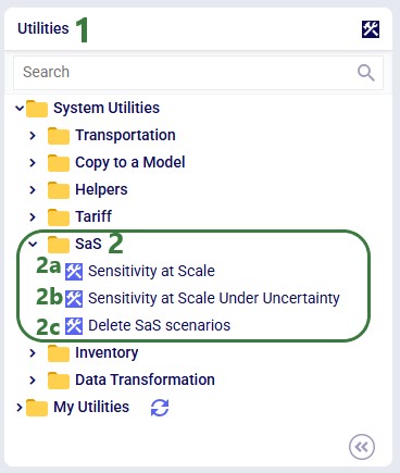
📝 Note: See the How to Use & Create Cosmic Frog Model Utilities Help Center article for details on using and building utilities.

Deleting Scenarios and Items

Select one or more scenarios or items, then right-click ? Delete or use the Delete option from the Scenario drop-down menu at the top of the module. Key behaviors to keep in mind:

1. Deleting a scenario item removes it from every scenario it belongs to.
2. Deleting only a scenario (none of its items) moves any items no longer used by other scenarios to the Unassigned Items folder.
3. Deleting a scenario also deletes all its outputs.
4. Use the Ctrl key to select multiple scenarios and/or items. Use Ctrl + Shift to select a continuous set of scenarios and items.

Example: Deleting Scenarios Only

1. Ctrl-click two scenarios to select them (dark highlight).
2. At the bottom, it is summarized how many scenarios and items are currently selected.
3. No items are selected.

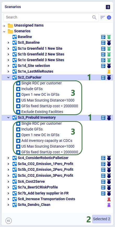
Deleting removes only the two scenarios. Items used exclusively by those scenarios move to Unassigned Items; items shared with other scenarios remain untouched.

Example: Deleting Scenarios and Items Together

1. Ctrl + Shift was held down to select a contiguous block of scenarios and all their items:
   • The use first clicked on the Sc2_CoPacker scenario.
   • Next, the user clicked on the Sc3_PrebuildInventory scenario.
2. This selects the 2 scenarios and all 6 scenario items of the Sc2_CoPacker scenario. Since 5 of those items are also used by the Sc3_Prebuild Inventory scenario, they are highlighted as selected there too.
3. The count of selected scenarios and items is 8: 2 scenarios and 6 items.

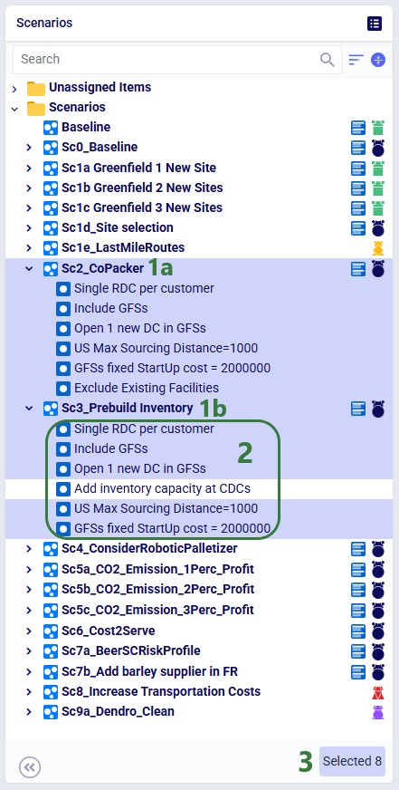
Deleting removes both selected scenarios and all 6 selected items - including from any other scenarios that use them. The one unselected item in these 2 scenarios, "Add Inventory capacity at CDCs", remains.

⚠️ Important: Deleting a scenario item removes it from all scenarios that it is assigned to, not just the selected scenario. Review item assignments before deleting.

Deleting Scenario Results

Use Delete Scenario Results (context menu or Scenario drop-down) to clear output data for one or more scenarios without removing the scenarios themselves:

1. After choosing Delete Scenario Results, the Delete Scenario Results panel comes up on the right-hand side.
2. Only scenarios that already have results are listed; use the Search box to filter by name.
3. The Sort icon orders by creation date ("Default") or alphabetically ("Name").
4. Use the top checkbox to select/deselect all (filtered) scenarios at once.
5. Use the individual checkbox to select/deselect a scenario.
6. The summary at the bottom shows total (16), filtered (3), and selected (2) scenario counts.
7. Click Delete to confirm or Cancel / x to abort.

Tips & Tricks

Naming Conventions

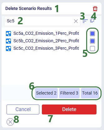
Think through scenario naming conventions ahead of time. You can for example:

1. Use a number prefix (S01, S02, etc.) to control scenario sort order in output tables, charts, and graphs.
2. Keep names short so they display fully when comparing scenarios side-by-side in charts.

Use Status + Notes for Scenario-Specific Records

Most input tables include Status and Notes fields. A powerful scenario pattern is:

1. Add scenario-specific records to a table with Status = Exclude and a Notes tag (e.g., 'Scenario 3').
2. Create a scenario item that sets Status = 'Include' where Notes = 'Scenario 3'.

This keeps all data in the model without interfering with the Baseline.

Use Custom Columns for Scenario Data

Custom columns let you store alternative values in a table and reference them in scenario items, e.g.:

1. A custom column on the Transportation Policies table named "newcost" contains updated cost numbers. A scenario item can then set unitcost = newcost, so that the scenario uses the numbers from the newcost column as the transportation costs.
2. A custom column on the Customer Demand table named "projection" contains growth percentages for demand quantities (e.g. 10 for 10%). A scenario item can then set quantity = quantity * (1 + (projection/100)) to apply those growth percentages in a scenario.

Copy Scenarios Between Models

The Copy Scenarios utility (Utilities module → Copy to a Model) copies a single scenario or all scenarios from one model to another, including all items and assignments.

Use Leapfrog AI

Use Leapfrog for scenario and item creation, and also for manipulating scenario-specific data.

Leapfrog can create scenarios and scenario items from a plain-language description - ideal for quickly spinning up variations without manually configuring each item. See the specific section on this in the Getting Started with Leapfrog AI Help Center article.

🔧 Leapfrog Use Case: 2026 Demand Projections from 2025 Numbers

Model 2026 demand from 2025 quantities using a custom growth projections table. Leapfrog can be utilized to set this up, so no external tool needs to be used:

1. Use Leapfrog to copy the 2025 demand record set into the Customer Demand table as a new set. Set Status = Exclude and Notes = '2026 Scenarios' for the copied records.
2. Use Leapfrog to update the dates of those records to 2026 (if date fields are used in the original demand data, otherwise not needed).
3. Use Leapfrog to multiply the demand quantities by the growth factor from the custom projection table, matching the tables on product and customer names.
4. In each 2026 scenario, use scenario items that set the Status of the 2025 records to Exclude and of the '2026 Scenarios' records to Include.

‍

Happy scenario modeling! As always, please contact our Support team on support@optilogic.com for any questions or feedback.

What Is It

The Run Python task allows you to execute Python scripts within a DataStar macro. You select a script, define its inputs (arguments), and run it as part of your workflow. This is ideal when built-in tasks are insufficient or when you want to reuse existing Python logic.

Use Cases

The Run Python task is especially useful when:

• Bulk importing or exporting data into or out of a project sandbox.
• Reusing existing Python scripts for data transformation instead of rebuilding logic in DataStar.
• The user prefers Python over visual workflow construction.
• Enriching data using external APIs.
• Integrating advanced libraries (e.g., pandas, NumPy) for efficient data manipulation.

Configuration

This walkthrough uses the end state of the DataStar Quick Start: Creating a Task using Natural Language guide as a starting point. At that point, a raw_shipments table has been imported and a Run SQL task has produced a customers table with unique customers. We will use a Run Python task to transform customer names from the format CZ1, CZ10, CZ100 to Cust_0001, Cust_0010, Cust_0100 - ensuring alphabetical sort matches customer number order and aligning the prefix with other data sources. The transformation steps are:

1. Remove the "CZ" prefix.
2. Left pad the number with leading zeroes to 4 digits.
3. Add the "Cust_" prefix.

The screenshot below shows the "Change customer names" Run Python task added to the macro:

Code File

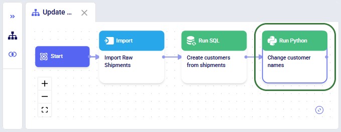
Once a Python task is added to the macro canvas, its configuration tab opens on the right:

1. Enter the task name here; in this example it is "Change customer names".
2. In the Code File section, choose File to select an existing .py file, or Template to use a pre-built script (covered in the Templates section).
3. Drag and drop a .py file from your local computer here to upload it to My Files/DataStar in your Optilogic account.
4. The list of .py files in your Optilogic account is shown here. The selected file (update_customer_names.py) is pinned to the top with a darker background so no scrolling is needed to see which file is selected.
5. The currently selected file is greyed out in the list (already selected).
6. Hover over a truncated column value to see its full text in a tooltip.
7. The file table is customizable:
   1. Drag column headers to reorder; click a header to sort (click again to reverse, third click removes sort; use Ctrl + Shift for multi-column sort).
   2. Click on the three-dot icon on a column header for a context menu with sort, pin, resize, and column visibility options.
   3. Drag the column divider to resize a column (the cursor changes to 2 arrows pointing away from each other).
8. Use the Search box to filter files by name.
9. After selecting a file, click on Use File to proceed to the next configuration step.
10. Click Create File to start a new script from scratch (see the Create File section).

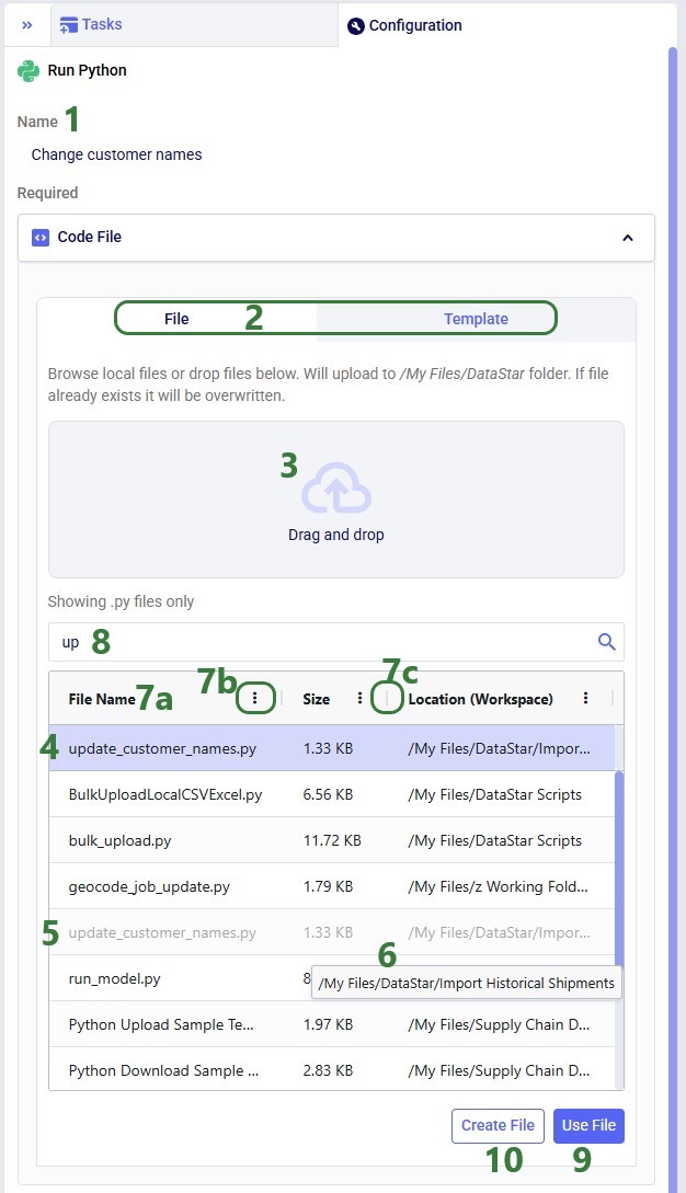
After clicking Use File with update_customer_names.py selected, the configuration updates as follows:

1. The selected file name is shown in the File Name field.
2. The file's path in your Optilogic account is shown in Directory Path.
3. Click Replace File to choose a different Python script.
4. Click Edit File to open the script in the Lightning Editor, another application on the Optilogic platform.
5. The Configure Python Arguments section allows an AI agent to auto-detect the script's arguments. The script needs to use the argparse module, see next section, for auto-detection to be possible. Note: auto-detection may occasionally be incorrect, and running it overwrites any previously configured arguments in the Command Arguments input of the Run Configuration section, see below.
6. Click Detect arguments to run the auto-detection.

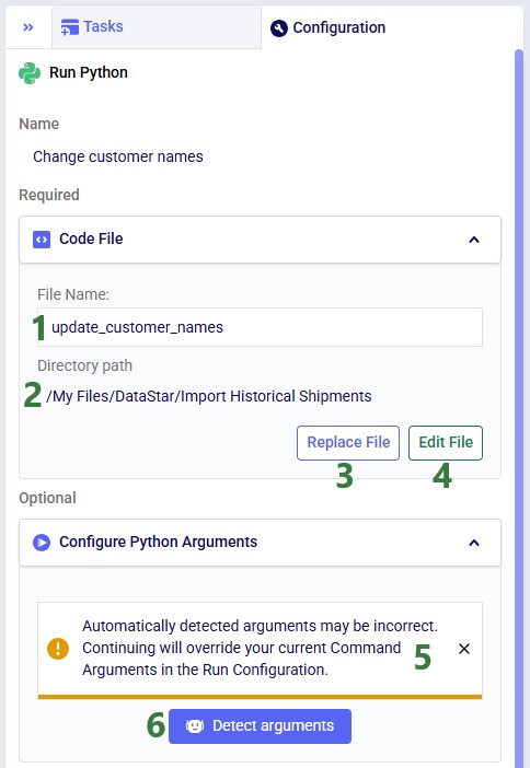
Before configuring arguments, we will cover the update_customer_names.py script. We can review its arguments so we can verify auto-detection is correct and look at the script body to understand what it does. You can copy the full script text from the Appendix.

1. Lines 1-2 import the argparse module (for parsing arguments) and the DataStar Python library (which also makes pandas available). See the Using the DataStar Python Library Help Center article for more details.
2. Line 4 begins the main() function - the conventional entry point for a script's logic.
3. Lines 5-12 define and call the argument parser:
   1. The description keyword briefly describes the script's purpose.
   2. Lines 8-10 define three required arguments (--project, --original_table, --column_name). Each has a name (double-dash prefix), a required flag, and a help string which will be shown as a tooltip in the DataStar UI when auto-detecting arguments.
   3. Line 12 parses the entered arguments; they are subsequently accessible as args.project, args.original_table, and args.column_name.
   4. Troubleshooting tip: add a print statement after line 12 to log parsed argument values to the Job Log (visible in the Run Manager application when a task is run). For example the statement print(f"project argument: {args.project}") will print the text "project argument: " followed by the value of args.project.
4. Lines 14-21 perform the data transformation using the DataStar Python library and pandas (which can be accessed after importing the DataStar library):
   1. Lines 14-17 connect to the project (--project), access its sandbox, read the --original_table into a dataframe (df_table), and copy it to df_new_table.
   2. Lines 18-20 transform the --column_name values: strip the "CZ" prefix, left-pad the number to 4 digits, and prepend with "Cust_".
   3. Line 21 writes df_new_table to the sandbox as a new table named new_<original_table_name>.
5. Line 23 prints a confirmation message to the Job Log once the script completes successfully.
6. Lines 25-26 call main() when the script is executed.

Configure Python Arguments and Run Configuration

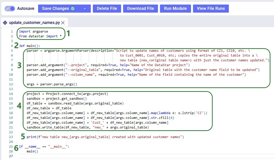
With the script understood, let us use Detect arguments and configure the task:

1. Three arguments are correctly detected. Their display names are derived from the key arguments of the argparse add_argument method.
   1. DataStar Project Name: type the name of the DataStar project to use.
   2. Original Table Name: type the name of the table containing the column with customer names that are to be updated. Hovering over the blue question mark shows the tooltip from the script's help key argument (see script screenshot above, line 9).
   3. Customer Name Column: type the name of the column containing the customer name values to be updated.
2. If the script changes, click the refresh button to re-run auto-detection of the script's arguments.
3. The Run Configuration section contains:
   1. Command Arguments: if auto-detection was not used, enter arguments manually here. When auto-detection is used, this field is read-only and shows the generated argument string.
   2. Tags: optionally, enter tags, which will be shown in the Run Manager jobs list and can help identify the job(s) of interest quickly.
   3. Timeout: the task is stopped if not completed within this many seconds. Default is 86,400 (24 hours).
   4. Resource Size: select the CPU/RAM size for the run. Larger resources have higher billing factors - see the Resource Size Selection Guide for more information.

Notes

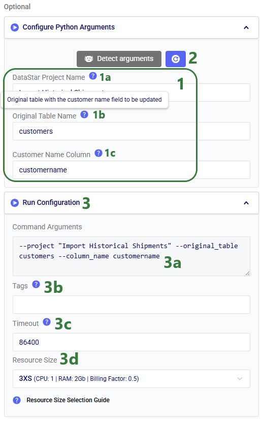
The Notes section is the final configuration area. It is especially valuable for complex tasks or collaborative projects, enabling users to quickly understand what the task does. Formatting options are available above the text box:

Running the Python Task

Before running the task, we examine the customers table in the sandbox:

1. Click the customers table in the sandbox to open it.
2. The customername column uses a CZ prefix and no leading zeros for the numbers, so values sort alphabetically by string rather than by customer number.

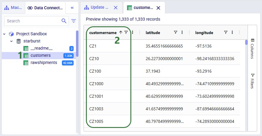
Now run the "Change customer names" task (hover over it on the macro canvas and click the play button) and examine the results:

1. A new table named new_customers has been created in the project sandbox. Click it to open.
2. Customer names now follow the Cust_XXXX format. Sorting by name now orders them by customer number.

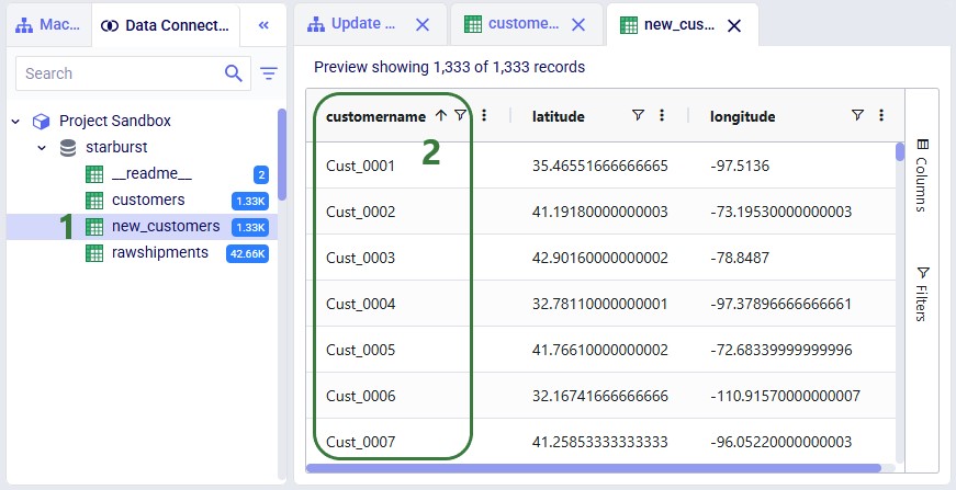
The Run Manager logs are useful for monitoring progress and troubleshooting:

1. Click the Run Manager icon in the left-hand application bar (scroll down or click the three-dot icon if not visible).
2. Find the Python task run in the job list - its Job Name matches the Python file name. Click it to see available logs on the right.
3. Click the report icon to open the Job Log.
4. Print statements in the script appear here. Use them throughout your script to track progress of long-running tasks.
5. If a job fails, click the hazard icon to open the Error Log which may contain helpful diagnostic information.

Create File

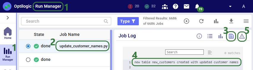
Instead of using an existing file, users can click the Create File button in the Code File area (see bullet 10 underneath the first screenshot of the Code File section) to create a new script directly on the Optilogic platform:

1. A new file named datastar-<timestamp>.py is created in My Files/DataStar in your Optilogic account.
2. Clicking the file opens it in the Lightning Editor application.
3. The file initially contains only print("Hello Datastar!"). Edit it to build your own script, and use for example the text of the script covered above, which can be copied from the Appendix, as a starting point.

Templates

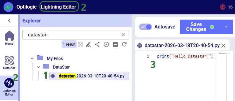
Templates are pre-built scripts available to all users from the Resource Library, covering common import/export patterns. To browse them, open the Resource Library application, filter for DataStar resources (button at the right top) and the Script tag. Clicking a resource also shows available documentation, which can be copied to your Optilogic account or downloaded.

1. Click on the Template tab in the Code File section.
2. Browse and select a template from the list. The same search and grid customization features apply here as in the File tab, see the Code File section above.
3. Click on the Use Template button to proceed:

1. A default file name based on the script name and current timestamp is used for the copy saved to your account.
2. The file is placed in /My Files/DataStar.
3. Click Replace File to choose a different script or Edit File to open the current file in the Lightning Editor.
4. If the selected Template does not use argparse, as is the case here, auto-detection of arguments is unavailable. Arguments (if any) must be entered manually in the Command Arguments field of the Run Configuration area. For this script, user-configurable values are set directly in the script's "User Configuration" section, and nothing needs to be entered in the Command Arguments field:

1. Open the Explorer application and locate the script under My Files/DataStar. Click it to open in the Lightning Editor.
2. The imports section shows which libraries the script uses. All these are included when running a Python file from your Optilogic account, so no requirements.txt is needed in this case.
3. User-configurable values are set directly in the "User Configuration" section of the script. Comments (green text) describe the expected inputs, and more information may be available in the documentation of the script on the Resource Library.

Requirements.txt File

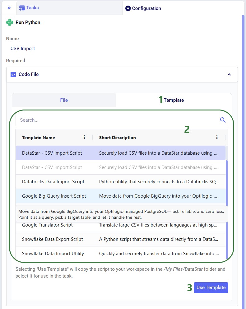
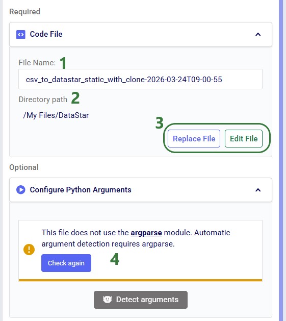
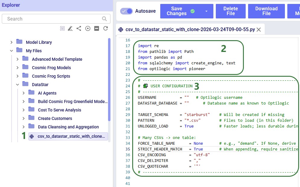
The Python base image used by the Run Python task contains the Python libraries most used in conjunction with DataStar. If your script uses a library that is not included in this base image, you need to create a requirements.txt file and place it in the same location as your Python script. In this file, you need to list the names of the libraries (without quotes), 1 library name per line.

If your script uses a library that is not part of the base image, the Job Error Log of the Python task run will contain the following error: "ModuleNotFoundError: No module named '<module name>'".

Tips & Tricks

Keep the following in mind when developing scripts for Run Python tasks:

• Consider whether to hard-code values or pass them as arguments. Hard-coded values make a script simpler but less reusable. Using arguments in our example script allows it to work across projects, tables, and columns. Think for example of needing to update the customer names in all raw data, including a "shipments" table where the "destination" field contains customer names.
• Use print statements throughout your script for troubleshooting. They appear in the Job Log and, possibly in combination with the Job Error log, help pinpoint where a script fails or stalls.
• Build and test incrementally - run the script after each sub-task is complete to catch issues early.
• Test scripts on copies of your data to protect the originals.
• When using uncommon Python libraries in your script, place a correctly populated requirements.txt in the same folder as the script. If this is not done, the Job Error Log will contain the following error: "ModuleNotFoundError: No module named '<module name>'".

Helpful Resources

• For more on DataStar, see the Navigating DataStar section on Optilogic's Help Center. Particularly relevant articles:
  • Using the DataStar Python Library
  • The 2 preceding quick starts to get to the point we started from in this documentation:
    • DataStar Quick Start: Importing a CSV File
    • DataStar Quick Start: Creating a Task using Natural Language
• Getting started with Python

As always, our Support team is happy to help with any questions; they can be reached at support@optilogic.com.

Appendix - Script Text

Copy the script below into a .py file in your Optilogic account (via the Lightning Editor) and modify it as needed:

import argparse
from datastar import *

def main():
    parser = argparse.ArgumentParser(description="Script to update names of customers using format of CZ1, CZ10, etc. \
                                                    to Cust_0001, Cust_0010, etc; copies the entire original table into a \
                                                    new table (new_<original table name>) with just the customer names updated.")
    parser.add_argument("--project", required=True, help="Name of the DataStar project")
    parser.add_argument("--original_table", required=True, help="Original table with the customer name field to be updated")
    parser.add_argument("--column_name", required=True, help="Name of the field containing the name of the customer")
    
    args = parser.parse_args()

    project = Project.connect_to(args.project)
    sandbox = project.get_sandbox()
    df_table = sandbox.read_table(args.original_table)
    df_new_table = df_table
    df_new_table[args.column_name] = df_new_table[args.column_name].map(lambda x: x.lstrip('CZ'))
    df_new_table[args.column_name] = df_new_table[args.column_name].str.zfill(4)
    df_new_table[args.column_name] = 'Cust_' + df_new_table[args.column_name]
    sandbox.write_table(df_new_table, "new_" + args.original_table)
    
    print(f"new table new_{args.original_table} created with updated customer names")

if __name__ == "__main__":
    main()

The following link provides a downloadable (excel) template describing the fields included in the output tables for Neo (Optimization), Throg (Simulation), Triad (Greenfield), and Hopper (Routing).

Anura 2.8 is the current schema.

• Anura 2.8 Output Documentation

A downloadable template describing the fields in the input tables can be downloaded from the Downloadable Anura Data Structure - Inputs Help Center article.

The best way to understand modeling in Cosmic Frog is to understand the data model and structure. The following link provides a downloadable (Excel) template with the documentation and explanation for every input table and field in the modeling schema.

• 2.8 Anura Input Documentation

A downloadable template describing the fields in the output tables can be downloaded from the Downloadable Anura Data Structure - Outputs Help Center article.

For a brief review of how to use the template file, please watch the following video.

If you are seeing a "Something went wrong" error when trying to open a model in Cosmic Frog — for example, Cannot read properties of undefined (reading 'call') — this is likely caused by a cached version of the application conflicting with a recent platform update. Follow the steps below in order to resolve it.

Step 1: Hard Refresh

A hard refresh forces the browser to bypass its cache and reload all files directly from the server. It clears the cache for that specific page only and ensures the latest version is loaded. This is the quickest fix for pages that have not updated properly and should be tried first.

Press the following keyboard shortcut to perform a hard refresh:

• ‍Windows: Ctrl + Shift + R ‍
• Mac: Cmd + Shift + R

Once the page has reloaded, try opening your model again.

Step 2: Clear Browser Cache

If the hard refresh does not resolve the issue, clearing your full browser cache will remove all stored files and force the browser to fetch the latest version of Cosmic Frog from the server.

Opening the Clear Browsing Data menu

Press the following keyboard shortcut to open the Clear Browsing Data menu:

• ‍Windows: Ctrl + Shift + Del ‍
• Mac: Cmd + Shift + Del

Clearing the cache

In the menu that appears:

1. Check the box for Cached images and files
2. Set the time range to All time
3. Click Clear data

Once cleared, refresh the Cosmic Frog page and try opening your model again.

Still Experiencing Issues?

If neither step resolves the problem, please contact the Optilogic support team. Include your browser type and version, and a screenshot of the error if possible.

Email: support@optilogic.com

‍

In this quick start guide we will walk-through importing a CSV file into the Project Sandbox of a DataStar project. The steps involved are:

1. Creating a CSV Data Connection
2. Adding an Import Task that takes the data from the CSV file and imports it into the Project Sandbox through a Macro

Our example CSV file is one that contains historical shipments from May 2024 through August 2025. There are 42,656 records in this Shipments.csv file, and if you want to follow along with the steps below you can download a zip-file containing it here (please note that the long character string at the beginning of the zip's file name is expected).

Creating a CSV Data Connection

Open the DataStar application on the Optilogic platform and click on the Create Data Connection button in the toolbar at the top:

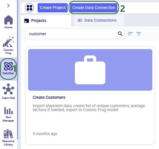
In the Create Data Connection form that comes up, enter the name for the data connection, optionally add a description, and select CSV Files from the Connection Type drop-down list:

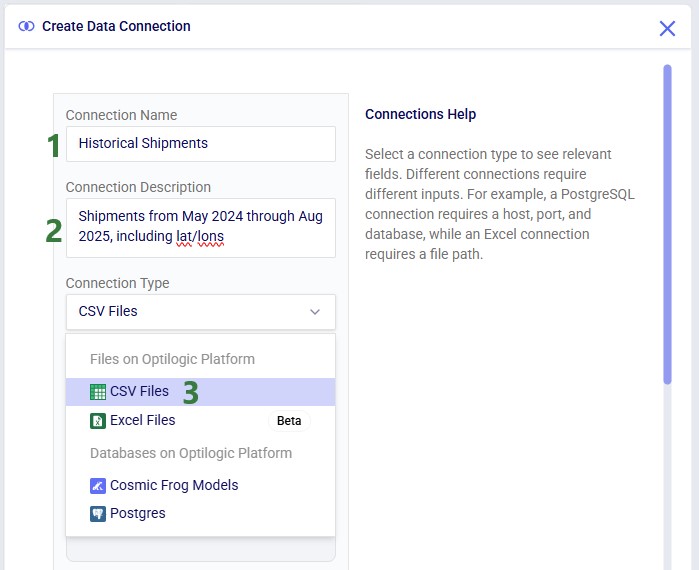
If your CSV file is not yet on the Optilogic platform, you can drag and drop it onto the “Drag and drop” area of the form to upload it to the /My Files/DataStar folder. If it is already on the Optilogic platform or after uploading it through the drag and drop option, you can select it in the list of CSV files. Once selected it becomes greyed out in the list to indicate it is the file being used; it is also pinned at the top of the list with darker background shade so users know without scrolling which file is selected. Note that you can filter this list by typing in the Search box to quickly find the desired file. Once the file is selected, users can optionally configure additional settings available on the right-hand side of the form, see the CSV File Data Connection help center article for details on these configuration options. Finally, clicking on the Add Connection button will create the CSV connection:

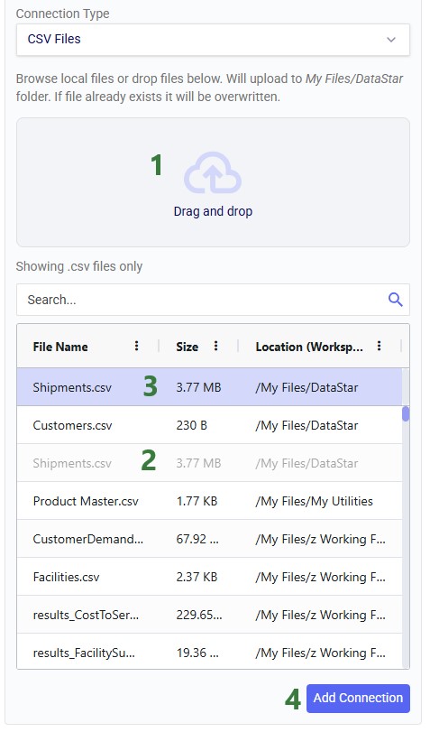
After creating the connection, the Data Connections tab on the DataStar start page will be active, and it shows the newly added CSV connection at the top of the list (note the connections list is shown in list view here; the other option is card view):

Importing a CSV File into the Project Sandbox

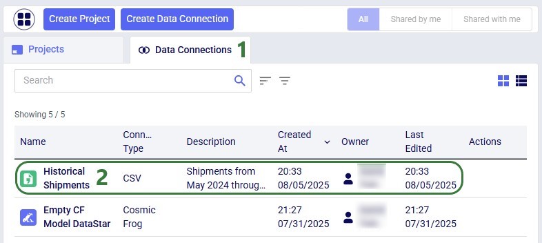
You can either go into an existing DataStar project or create a new one to set up a Macro that will import the data from the Historical Shipments CSV connection we just set up. For this example, we create a new project by clicking on the Create Project button in the toolbar at the top when on the start page of DataStar. Enter the name for the project, optionally add a description, change the appearance of the project if desired by clicking on the Edit button, and then click on the Add Project button:

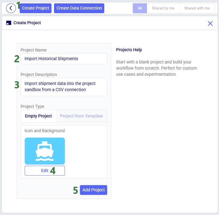
After the project is created, the Projects tab will be shown on the DataStar start page. Click on the newly created project to open it in DataStar. Inside DataStar, you can either click on the Create Macro button in the toolbar at the top or the Create a Macro button in the center part of the application (the Macro Canvas) to create a new macro which will then be listed in the Macros tab in the left-hand side panel. Type the name for the macro into the textbox:

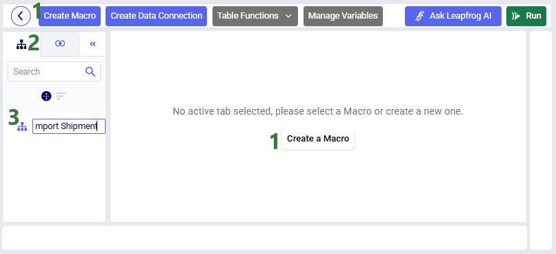
When a macro is created, it automatically gets a Start task added to it. Next, we open the Tasks tab by clicking on tab on the left in the panel on the right-hand side of the macro canvas. Click on Import and drag it onto the macro canvas:

When hovering close to the Start task, it will be suggested to connect the new Import task to the Start task. Dropping the Import task here will create the connecting line between the 2 tasks automatically. Once the Import task is placed on the macro canvas, the Configuration tab in the right-hand side panel will be opened. Here users can enter the name for the task, select the data connection that is the source for the import (the Historical Shipments CSV connection), and the data connection that is the destination of the import (a new table named “rawshipments” in the Project Sandbox):

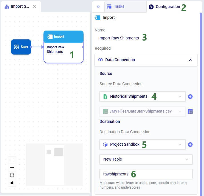
If not yet connected automatically in the previous step, connect the Import Raw Shipments task to the Start task by clicking on the connection point in the middle of the right edge of the Start task, holding the mouse down and dragging the connection line to the connection point in the middle of the left edge of the Import Raw Shipments task. Next, we can test the macro that has been set up so far by running it: either click on the green Run button in the toolbar at the top of DataStar or click on the Run button in the Logs tab at the bottom of the macro canvas:

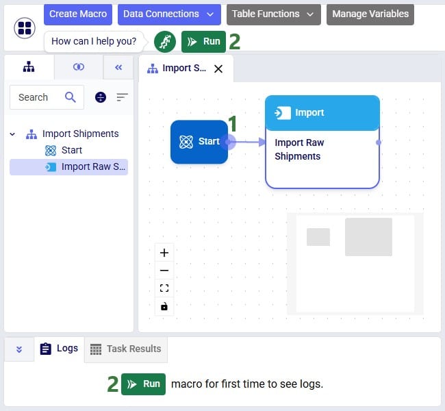
You can follow the progress of the Macro run in the Logs tab and once finished examine the results on the Data Connections tab. Expand the Project Sandbox data connection to open the rawshipments table by clicking on it. A preview of the table of up to 10,000 records will be displayed in the central part of DataStar:

Helpful Resources

• All available DataStar documentation on Optilogic's Help Center can be found here in the "Navigating DataStar" section.
• DataStar specific resources such as scripts for uploading data and connecting to external data sources, and template projects can be found on the Resource Library. To filter for DataStar related resources, click on the DataStar button at the top right.

‍

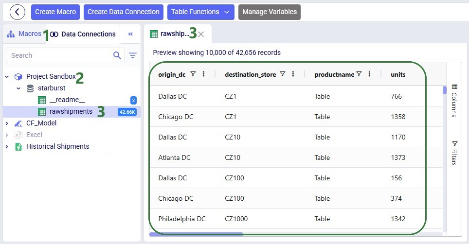
Please watch this 5-minute video for an overview of DataStar, Optilogic’s new AI-powered data application designed to help supply chain teams build and update models & scenarios and power apps faster & easier than ever before!

For detailed DataStar documentation, please see Navigating DataStar on the Help Center.

This documentation covers how to create and configure DataStar CSV File data connections.

Selecting your Data Source File

After opening DataStar, you can use the Create Data Connection button to add new data connections which can be used by all your DataStar projects:

1. On the DataStar start page, click on the Create Data Connection button which opens the Create Data Connection form.
2. Type the name for the connection in the Connection Name text box.
3. Optionally, add a description for the connection in the Connection Description text box. Especially when working with lots of data files and/or collaborating with others, descriptions can be helpful to understand quickly what data is contained in a connection.
4. Choose the Connection Type from the drop-down list. Options are CSV Files, Excel Files, Cosmic Frog Models, and Postgres Databases. This documentation focuses on the CSV Files connection type.
5. You can either choose a CSV file already present in your Optilogic account from the list below or drag and drop a file from your local computer on top of this "Drag and Drop" area to upload it to the My Files/DataStar folder in your Optilogic account.
6. When uploading a file through the drag and drop option, a message confirming successful upload appears here once the upload has completed.
7. To quickly find the file you want to use for the connection, use this free type Search text box to find CSV files in your account that contain the typed text in their file names.
8. After clicking on a file in the list, it will appear at the top of the list with a colored background. This is so users can easily see which file they have selected as the file itself could be much further down the list.
9. The selected file will be greyed out in the list and cannot be clicked on, since it is already the actively selected file.
10. The list of files contains 3 columns: File Name, Size, and Location. Users can click on the column headings to sort the list by the column's values. Use Ctrl + Shift to sort by multiple columns. Columns can also be resized and dragged to change their order. Click on the 3 vertical dots to bring up a context menu from which additional options for sorting, pinning, auto-sizing, and choosing columns can be accessed.
11. Once the user has configured the parameters on the right-hand side of the form (not shown in the above screenshot; covered in the screenshots that follow), clicking on the Add Connection button will create the connection.

Configuration Options

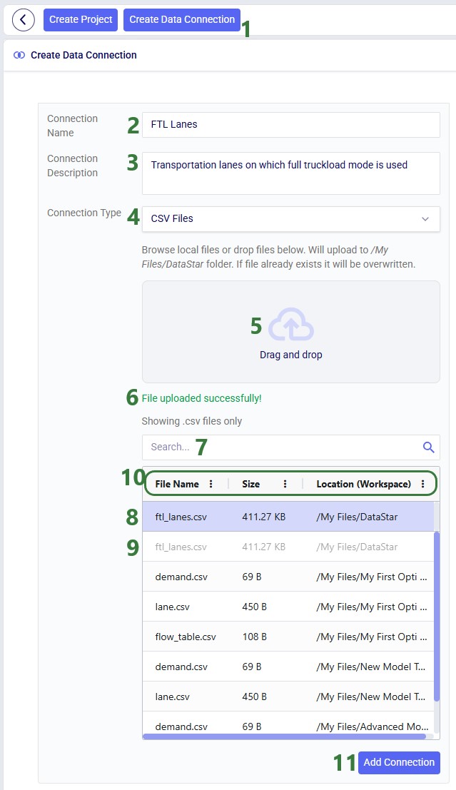
On the right-hand side of the Create Data Connection form, configuration options for the creation of the CSV File data connection are available. These will be covered now using the following screenshots.

Parameters

1. There are 3 different configuration sections; each can be expanded or collapsed by using the caret icon to the left of the section's name.
   1. Parameters - setting these appropriately ensures the data in the CSV file is interpreted correctly.
   2. Column Selection - this allows users to choose a subset of columns to be imported and to change names and data types of columns.
   3. Data Preview - users can see a preview of the data that will be contained in the data connection.
2. Record Limit (Optional) - if not set or left at the default of 0, all records of the CSV File will be part of the data connection. When setting a limit, for example a limit of 1,000, only the first 1,000 records of the CSV file will be part of the data connection.
3. Delimiter - choose the character that functions as the character indicating where a column ends and the next begins from the drop-down list. This is most commonly a comma (the default) for CSV files but needs to be updated in case a different character is used.
4. Thousand Separator - choose the character that is used in the data in the CSV file in numbers over a thousand, in between the 3^rd and 4^th digit (counting from the first digit before the decimal separator).
5. Decimal Separator - choose the character that is used in the data in the CSV file in between the last integer digit and first decimal digit.
6. First Record contains Column Names - when toggled on (the default), the data in the first record in the CSV file will be used as the column names. When off, the columns will be named column_1, column_2, etc., and the first record of the file becomes the first data record in the data connection.
7. Quote Character - choose the character that is used in the data around string values.
8. Null Values (comma-separated) - indicate what values in the data should be interpreted as null values. If more than one, use a comma in between them.

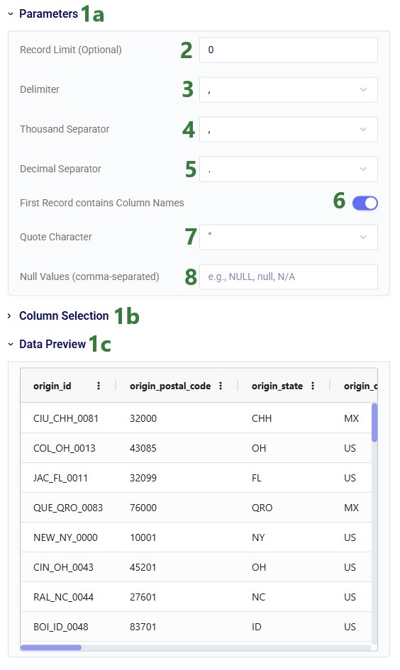
Note that when making any changes in these parameters the Data Preview below is immediately updated to take those changes into account. This is helpful to ensure that the parameters are set correctly.

Column Selection

Next, we will look at the Column Selection area, which was collapsed (the default) in the previous screenshot, but is expanded in the next one:

1. Selection - using these checkboxes, users can indicate which columns to use in the Data Connection. Use the checkbox at the top to simultaneously enable or disable all checkboxes of all columns.
2. Column Name and New Column Name - this first column shows the name of the column in the original CSV file. In the second column, users can overwrite this original name by typing in a new name. This new name will be used as the column name in the data connection.
3. Data Type - the current data type of the column is shown here: t for text, n for number, b for Boolean, and d for date. The data type can be changed to a different one by selecting the new data type from the drop-down list, see the next screenshot.

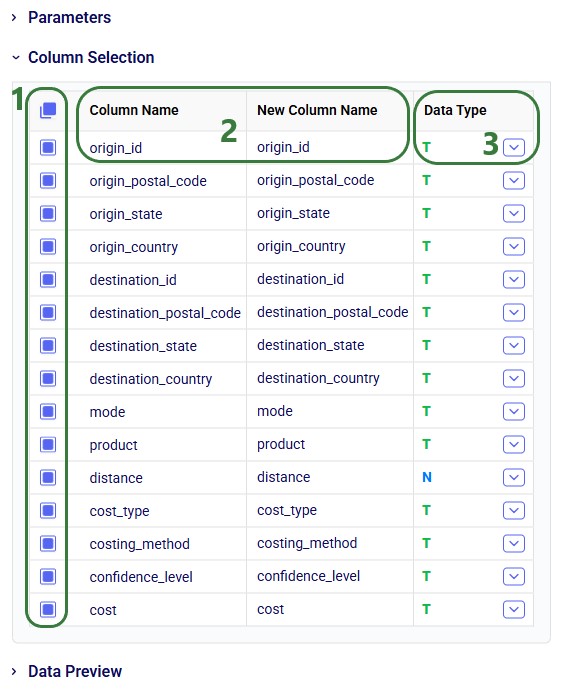
The drop-down list that comes up when clicking on the caret icon in a data type field is shown in this screenshot:

1. Open the drop-down list by clicking on the caret icon.
2. To quickly find the data type of interest, users can type part of the name of the data type they are looking for in this Search text box.
3. Part of the list of available data types is shown here. Note that multiple different text, number, and date types are available.

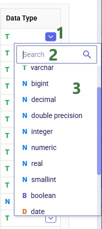
Just as with the Parameters section, making changes in this Column Selection section updates the Data Preview automatically.

Data Preview

Finally, the Data Preview section shows a preview of the data as it is currently configured based on the Parameters and Column Selection sections:

1. The Data Preview section is expanded.
2. You may need to use the horizontal and vertical scroll bars to see the whole Data Preview.
3. The column order can be changed by dragging and dropping the column headers. The data can also be sorted by clicking on the column headers. To sort by multiple columns, hold down Ctrl + Shift when clicking on the column headers that you want to sort by.
4. Click on the icon with 3 vertical dots to bring up a context menu which gives access to additional column sort, pin, auto-size, and selection options.
5. To adjust column width, hover over the vertical field divider until the cursor becomes 2 arrows pointing away from each other, then click and move the cursor left or right to make the field narrower or wider.

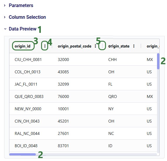
Once the configuration of the data connection is finalized, click on the blue Add Connection button, shown in the first screenshot above, to create the CSV data connection.

Other Helpful Resources

Learn all about DataStar from the Navigating DataStar section on Optilogic's Help Center.

We are excited to announce the upcoming release of Anura schema version 2.8.19, with enhancements to our engines and model run options. The migration rollout will start soon and is expected to be completed by the end of March.

All updates in this release are additive — there are no breaking changes.

🔧 Major Projects Enabled by This Release

‍Neo

• Process yield modeling - Processes can have a yield % where some product is lost during production.

Hopper

• Compartment modeling - Products can be placed in compartments within a single shipment, enabling compartment-specific constraints.

Other

• Utility Curves for easily specifying Dendro parameters
• Improvements to plotting road networks in Cosmic Frog

Model Run Options

• New Neo MRO: MaxNumberOfSourcesToConsiderForMultiStopRoutes
  • When Hopper is called inside NEO, it creates multi-stop routes for shipments from a source to multiple destinations. This option limits the top closest sources for each customer that Hopper will consider when creating these multi-stop routes. A higher number of sources may lead to better optimization of routes but can also increase computational time and resource usage.
• New Dendro MRO: DendroTimeout
  • Time in seconds after which the system will cancel a Dendro generated simulation. This is helpful in case runs get stuck to prevent blocking the next generation. Best practice is to set the time at 1.25-1.5 X the time it takes to simulate the Baseline.

CYCLO - Multi-Echelon Inventory Optimization

• Some of these schema changes are in anticipation of the release of Cyclo (expected towards the end of Q2) - a brand new engine that optimizes on-hand inventory at all locations and can be used in conjunction with Dendro.

📋 New Schema Objects

🆕 6 New Tables

• CompartmentConfigurations
• InventorySettings
• UtilityCurves
• InventoryNetworkSummary
• InventorySafetyStockSummary
• InventoryValidationErrorReport

📈 7 New Columns Across Existing Tables

• TransportationAssets.CompartmentConfigurationName
• TransportationPolicies.MaximumServiceTime
• TransportationPolicies.MaximumServiceTimeUOM
• TransportationPolicies.MinimumServiceTime
• TransportationPolicies.MinimumServiceTimeUOM
• OptimizationProcessSummary.DisposalBehavior
• TransportationShipmentSummary.CompartmentName

If you have any questions or concerns about this upcoming Anura upgrade, please reach out to Optilogic Support at support@optilogic.com.

What is Infeasibility?

When a scenario run is infeasible, it means that the solver cannot find any solutions that satisfy all the specified constraints simultaneously. In other words, the defined constraints are too restrictive or they contradict each other, making it impossible to satisfy all of them at once. Examples are:

• Total initial inventory + production capacity over a model's horizon are 12.5M units and the total demand is for 13M units
• Total flow using Mode = Rail is restricted to 150,000 lbs, but the destinations which only have Mode = Rail available to them need to receive at least 250,000 lbs in order to be able to satisfy all the demand in the model

Identifying an Infeasible Neo Scenario

If a Neo (network optimization) scenario run is infeasible, a user can tell from within Cosmic Frog and also by looking at the run's logs in the Run Manager application. Within Cosmic Frog, the Optimization Network Summary output table will show Solve Status = Infeasible and many other output columns, such as Solve Type and Solve Time, will be blank:

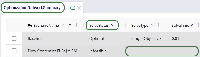
In the Run Manager application, also on the Optilogic Platform, users can select the scenario run, which will have Status = Error, and look at the run's logs on the right-hand side:

1. Click on the Run Manager button in the list of applications on the left-hand side while logged into the Optilogic platform (optilogic.app) to open the Run Manager application. If the Run Manager button is not visible, you may need to scroll or click on the button with 3 horizontal dots to show all applications.
2. Select the run for which you want to view the logs by clicking on the round checkbox. Here the user has selected the scenario run that was infeasible.
3. On the right-hand side multiple logs of the run are available. Clicking on the second icon will bring up the Job Records log.
4. The second entry in the Job Records log indicates that this run was infeasible.

Check Infeasibility Tool

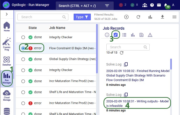
Running the check infeasibility tool is a great first step in identifying why a scenario is infeasible. It can allow the scenario to optimize even if the current constraints cause infeasibility. Generally, the tool will loosen constraints in the scenario, which allow it to solve. This means that the check infeasibility tool is solving an optimization problem focused on feasibility, not cost. The goal of this augmented model is to minimize how much the constraints are loosened, and therefore the tool can often find:​

1. Which constraints are violated, and​…
2. By how much

Running the Tool

The Check Infeasibility tool is accessed via the model run options on the Run Settings screen:

1. After clicking on the green Run button at the right top in Cosmic Frog, the Run Settings screen comes up.
2. Select the scenario you want to run the "Check Infeasibility" tool on.
3. On the right-hand side in Technology Parameters > Optimization (Neo), check the box of the Check Infeasibility tool to use it. Then click on the green Run button to kick off the infeasibility check.

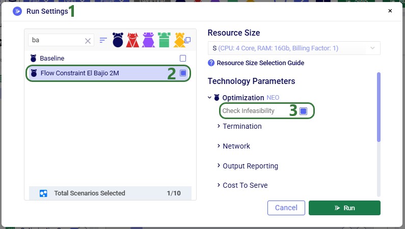
When running the Check Infeasibility tool in this default manner, all constraints will be relaxed. Additional run parameters can be used to selectively choose which constraints can be relaxed during a Check Infeasibility run and which need to be enforced, see the "Infeasibility Parameters" section in the "Running Models & Scenarios" help center article. Especially in models where many different types of constraints are applied, this can help in determining which constraint(s) cause the infeasibility and how constraints interact with each other. An approach can be to run the Check Infeasibility tool a few times with different constraints enforced and then compare the results. It also lets users indicate to the solver which constraints are most important to satisfy by keeping those enforced, while others are allowed to be relaxed.

1. Print Full Solution During Infeasibility Diagnosis - when this option is turned on, the full solution of the model during an infeasibility diagnosis run will be printed. This includes standard output tables (i.e. Optimization Network Summary, Optimization Flow Summary, Optimization Constraint Summary, etc.). This option only works when running the Check Infeasibility tool, which needs to be turned on. When this option is not turned on (the default), only the Optimization Constraint Summary output table is populated when running the Check Feasibility tool.
2. Relax … Constraints – when these options are turned on (by default they all are), the type of constraint described by the option's name will be allowed to be relaxed during a Check Infeasibility run. When turned off, the constraints of that type still need to be satisfied during a Check Infeasibility run.

Tool Output

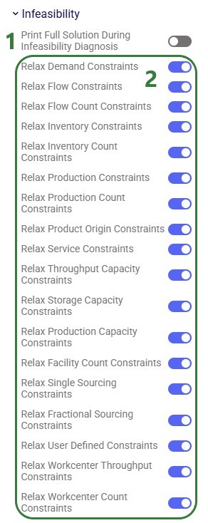
Once a Check Infeasibility run completes successfully, the results that are likely most helpful for identifying the infeasibility are found in the Optimization Constraint Summary output table. Users may need to filter for the scenario name in case this table contains results of multiple check infeasibility scenario runs. The following 2 screenshots show the 1 record in this table for the scenario called "Flow Constraint El Bajio 2M" scenario that returns infeasible as shown above. This first screenshot shows that the constraint in question is a Flow constraint that is applied on the lanes from the El Bajio Factory to a group of DCs named DCs Con:

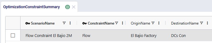
Scrolling right in the table, we can see additional fields which indicate why this constraint leads to infeasibility in the scenario:

1. The Constraint Type and Constraint Value fields repeat the type and value set for this constraint on the Flow Constraints input table, in this case a maximum flow of 2,000,000 was allowed.
2. The Constraint Violation and Suggested Constraint Value fields tell us by how much the original constraint (2M) needed to be violated (1,497,480) for the model to become feasible. Therefore, the suggested value for the constraint is 3,497,480 (2,000,000 original constraint + 1,497,480 constraint violation).

In this example, the check infeasibility tool can pinpoint the infeasibility exactly. At other times, the outcomes will be more general, see for example the following screenshots of results of a check infeasibility run on a different scenario:

Here the constraint that cannot be fulfilled is the demand for 1,000 units of Product_2 in Period_6. The output in the Constraint Summary output table is telling us that a way to make this feasible is to change the demand quantity to be 0. We will need to investigate the model inputs further to understand why this is. On further inspection, the infeasibility cause is found to be that the maturation time of Product_2 is set to 50 days. This is longer than the model horizon of 42 days (6 weekly periods). So, if no or not enough initial inventory is present in the model, Product_ 2 cannot be made and mature in time to fulfill demand in Period_ 6.

If the user has turned on the "Print Full Solution During Infeasibility Diagnosis" option, see above, the outputs in the other output tables can possibly also help to determine the cause of the infeasibility.

Final Notes

• Under certain circumstances, running the Check Infeasibility tool can still return infeasible, for example:
  
  • The tool was run with still enforcing a subset of the constraints and those by themselves cause the infeasibility
  • The model has numerical stability problems and the returned infeasibility is a false negative, it should have returned a feasible solution. A sign this could be the case is if the Constraint Summary output table does not contain concrete pointers to what causes the infeasibility. As a next step users could try separate runs where they change one of the following run parameters (one at a time).
    
    • Increase the MIP Relative Gap Percentage
    • Turn on Logical Constraints
    • Turn on Scale Input Data
• Sometimes, the cause of infeasibility is not immediately clear. Especially for more complex models with multiple constraints, infeasibility can be due to a combination of multiple different constraints.​
• In general, infeasibility is a complex topic. The check infeasibility tool cannot always catch or relax all potential infeasibility causes, but it is a very useful place to start.
• As always and especially if you cannot resolve an infeasible model yourself in a reasonable amount of time, please do not hesitate to contact the Optilogic support team at support@optilogic.com.

When a Cosmic Frog model has been built and scenarios of interest have been created, it is usually time to run 1 or multiple scenarios. This documentation covers how scenarios can be kicked off, and which run parameters can be configured by users.

Model Run Screen

When ready to run scenarios, users can click on the green Run button at the right top of the Cosmic Frog screen:

This will bring up the Run Settings screen:

1. We are on the Run Settings screen.
2. On the left-hand side of the screen a list of all scenarios contained in the model is shown. Users can select 1 or multiple of these to be run.
3. To facilitate finding specific scenarios in the list, text can be typed into the search box to filter the scenario list down to scenarios that contain the typed text in their name.
4. Clicking on this icon with the horizontal bars allows the user to sort the scenario list. Two sort options are available:
   1. Default: the scenarios are listed in the order they were added to the model (i.e. the same order as they are in in the Scenarios module).
   2. A-Z Name: this sorts the scenario list in alphabetical order. Clicking on this sort option again results in sorting the list in reverse alphabetical order.
5. These are the 5 icons associated with each of the Cosmic Frog engines. From left to right: network optimization (Neo), simulation (Throg), inventory (Dendro), Greenfield (Triad), and transportation optimization (Hopper). These icons are shown here for reference only.
6. The checkbox at the top of the scenario list can be used to check / un-check all scenarios that are showing in the list simultaneously.
7. Each scenario has an icon in front of it to show which engine will be used to run this scenario. These match the ones discussed under bullet number 5. The 2 scenario icons outlined in green are a Greenfield and a network optimization scenario, respectively. The other scenario icon outlined in green further down the list is an inventory scenario.
8. At the bottom of the scenario list the number of selected scenarios is listed. Here none are selected yet.
9. The user can select the Resource Size that they deem most appropriate for the scenarios to be run with. Larger resource sizes have more CPUs and more RAM available; however, they also have higher billing factors. Therefore, the aim is usually to choose a resource size as small as possible to limit the time billed for running the scenarios, while still being large enough for the scenarios to not run out of memory. More guidance on Resource Size selection and assessment can be found in this help article "Resource Size Selection Guidance"; a link to this article is provided underneath the drop-down list too.
10. For each engine, run parameters are available for configuration by users. We will go through these for each engine in the following sections of this documentation. Note that no parameters are available here for Greenfield runs; parameters to run Greenfield scenarios are all specified in the Greenfield Settings input table, which are covered in this "Greenfield Settings Explained" Help Center article.
11. When ready to start running the selected scenario(s), the user can click on the Run button. Note that it is now greyed out and unavailable as no scenarios have been selected. It will be available and green when 1 or more scenarios are selected.
12. Should the user decide to not run any scenarios at this time, they can close the Run Settings screen without kicking off any runs in 2 ways:
    1. By clicking on the Cancel button. If changes were made to any parameters, these changes will not be saved. In other words, the parameter values will be reverted to those that were there when the Run Settings screen was opened.
    2. By clicking on the x-icon at the right top of the Run Settings screen. If changes were made to any parameters, these changes will be saved.

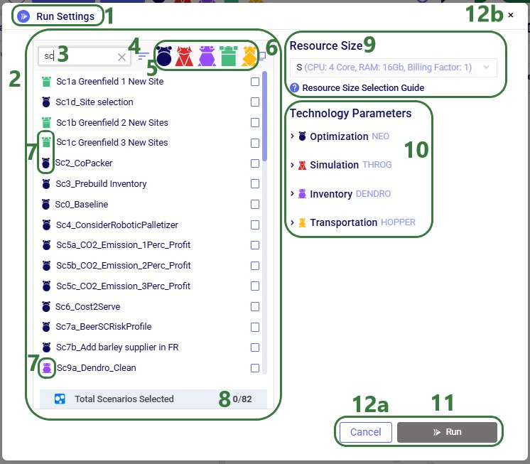
Please note that:

• Scenarios which are run with the same engine will use the same set of parameters when kicked off simultaneously. Should there be a need to run scenarios with different parameters, users currently need to kick them off in separate batches.
• Scenarios that are run simultaneously, will currently all use the same selected resource size. Should there be a need to run scenarios using different resource sizes, users currently need to kick them off in separate batches. More to come in future releases!
• Users can check the progress of all runs in Optilogic's Run Manager application:

1. To open the Run Manager, click on the Run Manager icon with the vertical bars on the left-hand side of the screen while on the Optilogic platform.
2. If the Run Manager application is not showing on the left-hand side of the screen, find the icon with the 3 dots and click on it to show all available applications. Then click on Run Manager.
3. There are 4 jobs listed here which, from bottom to top, are the overall job "General Demo_V3 (neo)" of kicking off network optimization (Neo) scenarios in the model named General Demo_V3. Three scenarios have been kicked off and are currently still running as their State = "running": Sc1d_Site selection, Sc2_CoPacker, and Sc3_Prebuild Inventory.
4. There are 4 jobs listed here which, from bottom to top, are the overall job "General Demo_V3 (triad)" of kicking off Greenfield (Triad) scenarios in the model named General Demo_V3. Three scenarios have been kicked off and have finished running as their State = "done": Sc1a_Greenfield 1 New Site, Sc1b_Greenfield 2 New Sites, and Sc1c_Greenfield 3 New Sites.
5. There are 2 jobs listed here which, from bottom to top, are the overall job "General Demo_V3 (dendro)" of kicking off inventory (Dendro) scenarios in the model named General Demo_V3. One scenario has been kicked off and has not completed successfully as its State = "error": Sc9a_Dendro_Clean.
6. When selecting an individual job by clicking on the circle to the left of it, additional details of the run can be viewed on the right-hand side (not shown in screenshot). This includes job info, job (error) logs, job resource usage metrics, etc.
7. Not shown in the screenshot above, but if a user wants to end a run, for example in case it was kicked off accidentally or it has been running for a long time without finishing, the user can right-click on the job and choose "Cancel Job" from the context menu.

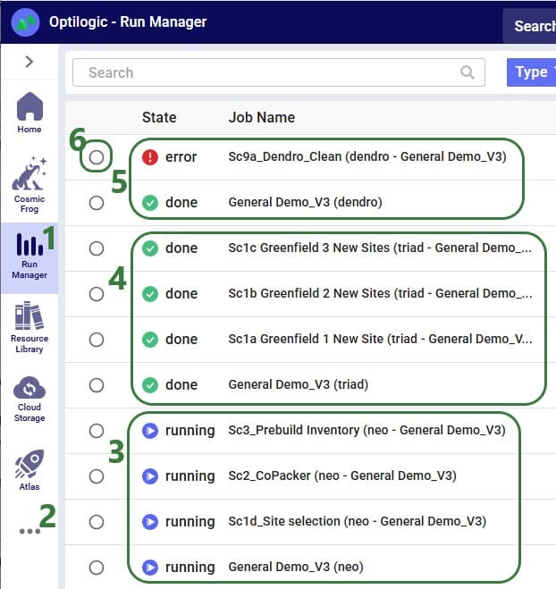
While we will discuss all parameters for each technology in the next sections of the documentation, please note that you can also find short explanations for each of them within Cosmic Frog: when hovering over a parameter, a tooltip explaining the parameter will be shown. In the next screenshot, the user has expanded the Termination section within the Optimization (Neo) technology parameters section and is hovering with the mouse over the "MIP Relative Gap Percentage" parameter, which brings up the tooltip explaining this parameter:

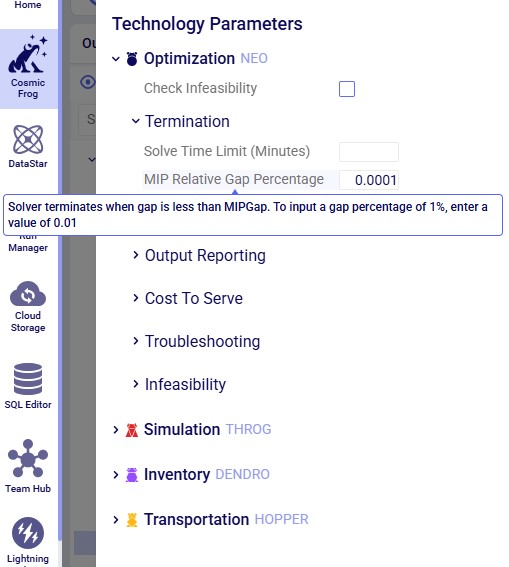
When selecting one or multiple scenarios to be run with the same engine, the corresponding technology parameters are automatically expanded in the Technology Parameters part of the Run Settings screen:

1. 3 scenarios are selected in the scenario list; they are all optimization (Neo) scenarios.
2. When one or multiple optimization scenarios are selected in the list, the Optimization section in the Technology Parameters part of the Run Settings screen is automatically expanded.
3. Users can manually expand/collapse these parameter sections by clicking on the caret icons.
4. In the Optimization section of the Technology Parameters part of the Run Settings screen, there is 1 general parameter (Check Infeasibility) and 6 additional categories of optimization parameters: Termination, Network, Output Reporting, Cost To Serve, Troubleshooting, and Infeasibility. These sections can also be expanded/collapsed using the caret icons. We will cover each section and their parameters in the next sections of this documentation.
5. Note that the Run button can now be clicked on and has turned green as 3 scenarios have been selected in the scenario list.

Optimization (Neo) Parameters

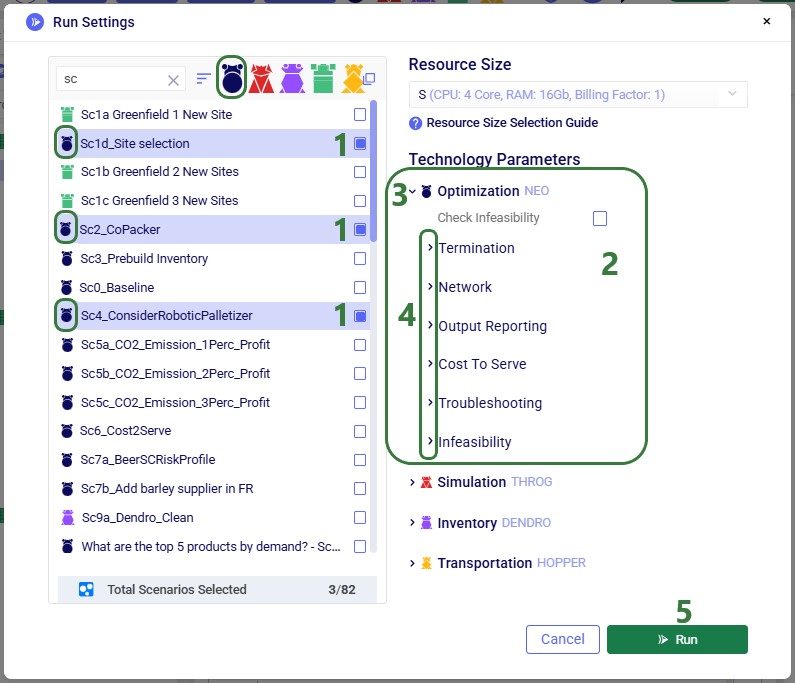
When enabled, the Check Infeasibility tool will run an infeasibility diagnostic on the model in order to identify any cause(s) of the scenario being infeasible rather than optimizing the scenario for minimal cost. For more information on using the check infeasibility tool, please see this Help Center article.

Optimization (Neo) – Termination Parameters

1. Solve Time Limit (Minutes) – specifies the maximum amount of time the scenario is allowed to run. This is set in minutes.
   1. If a feasible solution where the MIP Relative Gap Percentage (see bullet #2 below) has been reached is found before the Solve Time Limit is reached, the run will stop and this solution is returned. In this case the allowed time is not necessarily used up entirely.
   2. If the MIP Relative Gap Percentage has not been reached within the allowed time, but a feasible solution with a higher gap has been found, this solution will be returned.
   3. If no feasible solution has been found within the allowed time, the scenario run will end without returning results.
   4. The default is blank, meaning scenarios will run until a solution is found that reaches the MIP Relative Gap Percentage, see bullet 2 below.
   5. In case needed, scenarios can always be manually stopped by cancelling the job in the Run Manager application, as explained above.
2. MIP Relative Gap Percentage – once the difference (gap) between the best bound and currently best-found solution is less than this defined gap, the solver terminates, and the solution is returned as the solution. To set a value of 1%, enter 0.01. The default is set to 0.0001, meaning 0.01%.

Optimization (Neo) – Network Parameters

1. Lane Creation Rule – this parameter dictates how the transportation policies and sourcing policies (Customer Fulfillment Policies, Replenishment Policies, Procurement Policies, and Return Policies) input tables are used to create the lanes (origin-destination pairs) that are considered during the optimization. Options are:
   1. Transportation Policy Lanes Only: lanes are only created based on the origin-destination pairs specified in the Transportation Policies input table. This is the default setting for this parameter.
   2. Sourcing Policy Lanes Only: lanes are only created based on the origin-destination pairs specified in the Sourcing Policies input tables (which are: Customer Fulfillment Policies, Replenishment Policies, Procurement Policies, and Return Policies).
   3. Intersection: lanes are created for those origin-destination pairs that exist in both the Transportation Policies and Sourcing Policies input tables.
   4. Union: lanes are created for all origin-destination pairs that exist in the Transportation Policies table and the Sourcing Policies input tables.
2. Max Number Of Sources To Consider For Customers – when set, this adds constraints to the model where individual customers cannot source from more than this number of sources. It depends on the "Apply Max Number Of Sources By Location Only" parameter setting (see bullet 4 below) if this constraint is applied over the entire model horizon and over all products and modes together (the default behavior when this parameter is off) or for each product-mode-period combination at that location. The sources are evaluated based on distance. For example, if 5 sources are set up for a certain customer in the model, and this parameter is set to 2, then out of those 5 sources, only the 2 that are closest in distance to the customer are considered as sources. The default is blank, meaning that all sources that are set up in the model are kept.
3. Max Number Of Sources To Consider For Facilities – when set, this adds constraints to the model where individual facilities cannot source from more than this number of sources. It depends on the "Apply Max Number Of Sources By Location Only" parameter setting (see bullet 4 below) if this constraint is applied over the entire model horizon and over all products and modes together (the default behavior when this parameter is off) or for each product-mode-period combination at that location. The sources are evaluated based on distance. For example, if 3 sources are set up for a certain facility in the model, and this parameter is set to 1, then out of those 3 sources, only the 1 that is closest in distance to the facility is considered as a source. The default is blank, meaning that all sources that are set up in the model are kept.
4. Apply Max Number Of Sources By Location Only – when values are set for the previous 2 parameters, this parameter specifies if those max number of sources parameters are applied for each product-mode-period combination at that location or over all product-mode-period mode combinations together. When this parameter is off (the default), the max number of sources parameters will limit the number of sources for each destination across all product-mode-period combinations. When this parameter is turned on, the max number of sources parameters will limit the number of sources for each unique destination-product-mode-period combination.
5. Allow Cross Period Flows – turn this parameter on when flows that depart in one period and arrive in a later one need to be allowed in the model. This can be the case when (some) transport times are longer than the length of the periods in the model. By default, this parameter is off, and flows will depart and arrive in the same period regardless of the transport times specified in the model.
6. Open Close At Most Once – when turned on (the default), facilities and work centers which can be opened and/or closed during the model horizon are not allowed to change status more than once during the model horizon. When turned off, facilities and work centers are allowed to change between open and close states an unlimited number of times during the model horizon.
7. Keep Products Without Demand – when this option is turned off (the default), products for which no demand exists in the model will be entirely excluded from the model run. When turned on, these products will be included. This can affect the model results, for example:
   1. If there is initial inventory present for the product: inventory holding costs can be incurred and the product will take up storage space and count toward pre-build inventory.
   2. If there are min/fixed production or flow constraints for the product: these will need to be fulfilled, so production, transportation, and inventory holding costs can be incurred in this case, while the product also takes up space and counts towards pre-build inventory.
8. Keep Closest Lane For Max Sourcing – when this option is turned on (the default), if all sources where a max sourcing range is applied (set in the Max Sourcing Range fields of the Customer Fulfillment Policies, Replenishment Policies, and Procurement Policies tables) fall outside of this sourcing range, the closest source will be kept. When turned off, if all sources where a max sourcing range is applied fall outside of the range, this can lead to the model becoming infeasible if the destination location has no other way of receiving the product(s) it requires to fulfill demand or other model constraints.

Optimization (Neo) – Output Reporting Parameters

1. Print Detailed User Defined Variable Summary – when turned on, the Optimization User Defined Variable Summary and Optimization User Defined Variable Term Summary output tables are populated with all outputs related to user defined variables, including records with value of 0. When turned off (the default) these output table are only populated with non-0 values.
2. Print Constraint Summary – when turned on, the Optimization Constraint Summary output table will be populated, whereas when this parameter is turned off (the default) it will not be populated. As this table can contain a lot of records, it can be helpful to turn it off and only turn it on for troubleshooting purposes or for select scenarios to review how close some constraints are to maxing out for example.
3. Print Detailed Validation Error Report – when this option is turned off (the default), the Optimization Validation Error Report output table will group the found validation errors by type. When turned on, this table will have individual records for each instance of a validation error. For more information on the Validation Error Report output table, please see "Understanding the Validation Error Report" and "Troubleshooting with Validation Errors".
4. Generate Last-Mile Routes – when this option is turned on, the Hopper (transportation optimization) engine will be run once the Neo (network optimization) run is complete. This will generate last mile multi-stop routes based on the Neo assignments on this last leg and all Hopper output tables will be populated in addition to the Neo output tables. To learn more about this option to run "Hopper after Neo", please see "Network Transportation Optimization (Neo & Hopper)".

Optimization (Neo) – Cost To Serve Parameters

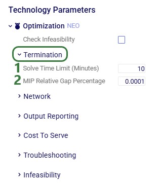
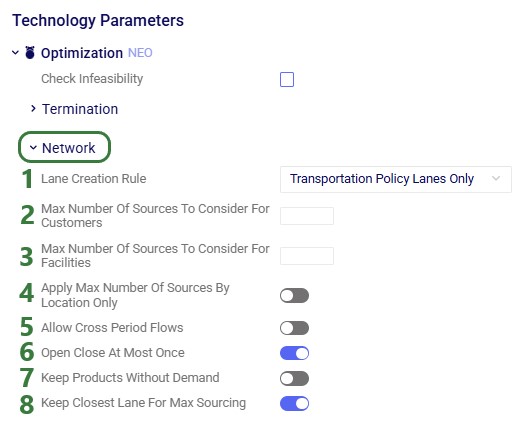
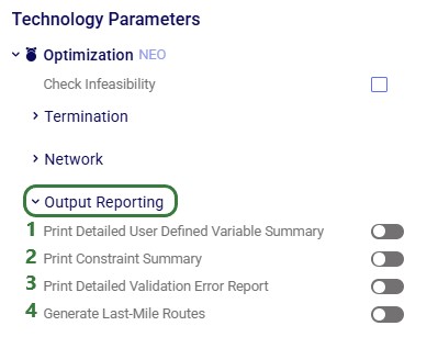
For more details on the Cost To Serve output tables that are populated by turning the options discussed below on, please see this "Cost to Serve Outputs (Optimization)" Help Center article.

1. Generate Cost To Serve Outputs – when this option is turned on (the default), the high-level Optimization Cost To Serve Summary output table will be populated after a scenario run. It is not populated when this option is turned off.
2. Generate Cost To Serve Path Data – when this option is turned on, the Optimization Cost To Serve Path Summary and Optimization Cost To Serve Path Segment Details output tables will be populated. Please note that:
   1. The "Generate Cost To Serve Outputs" option (see bullet 1 above) needs to be turned on when turning this option on.
   2. Turning this option on can add significant time to the output processing as many records may need to be generated for especially the Optimization Cost To Serve Path Segment Details output table, which affects the overall runtime of a scenario.

Optimization (Neo) – Troubleshooting Parameters

1. Feasibility tolerance – since numbers have finite precision on digital computers, sometimes constraints cannot be met exactly. Therefore, the feasibility tolerance sets a limit on the amount of violation allowed on a constraint while still considering it "satisfied". The default value is 0.000001, and for most models users will not need to change this. Should a user suspect a model turns infeasible due to slight constraint violation, they can test this out by relaxing the feasibility tolerance and setting it to a higher value, e.g. try 0.00001 first, then 0.0001, etc.
2. Write LP (linear program) File – when turned on, this will produce a file containing the linear programming formulation of the model that is being optimized. Experienced users may be able to review this for troubleshooting purposes, and Optilogic's support team may ask for this when troubleshooting any models. The LP-file can be found in the Explorer application: My Files > debug_data > model_name > scenario_name > NEO.lp. By default, this option is turned off. The next screenshot a bit further below shows where the NEO.lp file can be found when running a scenario with this parameter turned on.
3. Write Input Solver – when turned on, this will write all the data of the input tables that are used during the scenario run into .csv-files. This means that following have been applied before writing these files: scenario changes, excluded records are removed, and records using groups/named table filters are enumerated into records for the individual group/filter members (for groups used in constraints tables only if the group behavior field is set to enumerate). The .csv-files can be found in Explorer > My Files > debug_data > model_name > scenario_name > input_solver, see the screenshot a bit further below. By default, this option is turned off.
4. Relative Constraint Tolerance Percentage – constraints of type "Fixed With Tolerance" are relaxed by this amount. The default of 0.02 means a relaxation of 2%. For example, if a constraint of type "Fixed With Tolerance" is set to a constraint value of 500, then with a Relative Constraint Tolerance Percentage of 0.02 (2%), values from 490 up to 510 are accepted as satisfying the constraint.
5. Allow Lazy Constraints – when this option is turned on, constraints that are computationally expensive are at first turned off during the optimization and are added back in later in the process, so they are still respected in the final solution. By default, this option is turned off as it can slow the optimization down. Users are advised to turn it on when a performance issue is detected on a model, in which case it may be able to speed up the optimization.
6. Logical Constraints – if a model is poorly scaled (for example due to having both very small and very large demand quantities or cost numbers in it), turning this option on may prevent numerical issues leading to infeasibility of the model. Model runtime can however increase when this option is used. By default, this option is turned off.
7. Scale Input Data – when this option is turned on input data will be scaled; this can help to resolve numeric stability issues in models that contain a large range of numbers.
8. MIP Focus – the MIP Focus parameter allows you to modify your high-level solution strategy, depending on your goals. By default, the Gurobi MIP solver strikes a balance between finding new feasible solutions and proving that the current solution is optimal. If you are more interested in finding feasible solutions quickly, you can select MIP Focus=1. If you believe the solver is having no trouble finding good quality solutions, and wish to focus more attention on proving optimality, select MIP Focus=2. If the best objective bound is moving very slowly (or not at all), you may want to try MIP Focus=3 to focus on the bound.
9. Numerical Focus – the Numerical Focus parameter controls the degree to which the engine attempts to detect and manage numerical issues. The default setting (0) makes an automatic choice, with a slight preference for speed. Settings 1-3 increasingly shift the focus towards being more careful in numerical computations. With higher values, the code will spend more time checking the numerical accuracy of intermediate results, and it will employ more expensive techniques in order to avoid potential numerical issues.
10. Run Preprocessing Only – when this option is turned on, the scenario will first undergo preprocessing (i.e. applying scenario items, expanding groups into individual members, etc.) and then the Integrity Checker is run on the scenario. The results of the integrity checker can then be found in the Optimization Validation Error Report output table. No actual optimization is run when this option is turned on.

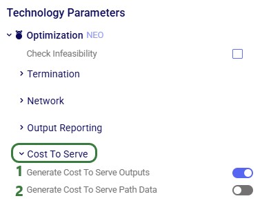
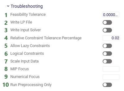
The following screenshot shows where the NEO.lp file can be found when running a scenario with the Write LP File parameter (bullet 2 under the above screenshot) turned on:

1. While in any application on the Optilogic platform, users can open/close the Explorer by clicking on the caret icon at the top left of the screen.
2. To quickly find the NEO.lp file, we can search for "debug" in the search box.
3. The file we are looking for is located in:
   
   1. The folder "My Files"
   2. The sub-folder "debug_data"
   3. The sub-folder with the name of the model, in this case "General Demo_V3"
   4. The sub-folder with the name of the scenario, in this case "Sc1d_Site selection"
4. The NEO.lp file in this folder is the file containing the linear programming formulation of this scenario.
5. The input_solver sub-folder contains the .csv files that are generated when the parameter "Write Input Solver" (see bullet 3 under the previous screenshot) is turned on.

Optimization (Neo) – Infeasibility Parameters

1. Print Full Solution During Infeasibility Diagnosis - when this option is turned on, the full solution of the model during an infeasibility diagnosis run will be printed. This includes standard output tables (i.e. OptimizationNetworkSummary, OptimizationFlowSummary, OptimizationConstraintSummary, etc.). This option only works when running the Check Infeasibility tool, which needs to be turned on (see further above). When not turned on (the default), only the Optimization Constraint Summary output table is populated when running the Check Feasibility tool on a scenario.
2. Relax … Constraints – when these options are turned on (by default they all are), the type of constraint described by the option's name will be allowed to be relaxed during a Check Infeasibility run. When turned off, the constraints of that type still need to be satisfied during a Check Infeasibility run. This can help users pinpoint infeasibility in models where many different types of constraints are applied and prioritize which constraints have to be adhered to vs others which may be nice to have satisfied. From the top, these constraints are specified in following input tables:
   1. Demand Constraints – Customer Demand and Facility Demand tables
   2. Flow Constraints – Flow Constraints table
   3. Flow Count Constraints – Flow Count Constraints table
   4. Inventory Constraints – Inventory Constraints table
   5. Inventory Count Constraints – Inventory Count Constraints table
   6. Production Constraints – Production Constraints table
   7. Production Count Constraints – Production Count Constraints table
   8. Product Origin Constraints – Customer Demand Origin Constraints table
   9. Service Constraints – Customer Transit Constraints table
   10. Throughput Capacity Constraints – Facilities table (Throughput Capacity field),
   11. Storage Capacity Constraints – Facilities table (Storage Capacity field)
   12. Production Capacity Constraints – Production Policies table (Production Rate field), Processes table (Processing Rate field), Suppliers table (Supplier Capacity field), and Suppliers Capabilities table (Supply Capacity field)
   13. Facility Count Constraints – Facility Count Constraints table
   14. Single Sourcing Constraints – Customers table (Single Source field, when set to True), Customer Fulfillment Policies table (Optimization Policy field, when set to Single Source), Replenishment Policies table (Optimization Policy field, when set to Single Source), Procurement Policies table (Optimization Policy field, when set to Single Source), Return Policies table (Optimization Policy field, when set to Single Destination)
   15. Fractional Sourcing Constraints –Customer Fulfillment Policies table (Optimization Policy field, when set to By Ratio), Replenishment Policies table (Optimization Policy field, when set to By Ratio), Procurement Policies table (Optimization Policy field, when set to By Ratio), Return Policies table (Optimization Policy field, when set to By Ratio)
   16. User Defined Constraints – User Defined Constraints table
   17. Workcenter Throughput Constraints – Work Centers table (Minimum Throughput and Throughput Capacity fields)
   18. Workcenter Count Constraints – Workcenter Count Constraints table

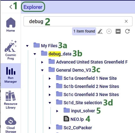
As more types of constraints are added to the Neo engine on an ongoing basis, not all may be captured by one of the above "Relax … Constraints" buckets. Any such constraints, like for example shelf life, are always relaxed when running the Infeasibility Check and, if they are the cause of infeasibility, reported in the Optimization Constraint Summary output table.

Simulation (Throg) Parameters

1. Number Of Replications – for simulation models that use variability in their inputs, multiple replications where different values are used for the variable inputs can be run. This can inform users on how robust a network is: out of all the replications run, how many show a well-functioning network in terms of cost, service and risk and how many do not? Running 20-30 replications is generally a good number to start with, keeping in mind that the more variable the input data is, the more replications should be used.
2. Run Replications in Parallel – when turned on, multiple replications will be run simultaneously rather than sequentially.
3. Log Progress – when turned on, a record will be printed in the job log of the simulation run for each day of the simulation horizon. See the next screenshot below on where to find this log. This can help users troubleshoot issues. For example, if a simulation run takes longer than expected, users can review the Job Log to see if it gets stuck on any particular day during the modelling horizon.
4. Confidence Interval Percent – the confidence interval used for calculating half-width statistics. The default is set to 0.95 (95%).
5. Cycle Stock Calculation Basis – this parameter controls how cycle stock is calculated for products in the model. If ReorderQuantity is selected (the default), the average cycle stock will be reported as ReorderQuantity / 2. If SafetyStock is selected, the average cycle stock will be reported as AverageInventory - SafetyStock.

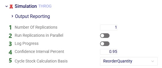
The following screenshot shows part of a Job Log of a simulation run, see also bullet 3 above:

1. Select the simulation run of interest in the Run Manager application on the Optilogic platform and choose to view the Job Log by clicking on the 4^th icon at the top right of the screen.
2. The current date and time are printed for each record printed in the Job Log.
3. The current simulation time is printed, a record for each day of the simulation is included.

Simulation (Throg) – Output Reporting Parameters

1. Inventory Reporting – choose whether and, if so, in what way the Simulation Inventory On Hand Report output table will be populated after a simulation run. Options are:
   1. End of Day Only: a record is printed for each facility-product combination at the end of each day.
   2. All Changes Only: a record is printed for facility-product combinations every time the inventory level changes.
   3. End of Day and All Changes: records are printed for each facility-product combination at the end of each day and also every time the inventory level changes. This is the default setting.
   4. None – the Simulation Inventory On Hand Report output table is not populated.
2. Print Order Report – when turned on (the default), the Simulation Order Report output table will be populated after a simulation run. This table tracks orders at all levels of the supply chain, e.g. production orders, replenishment orders, and customer orders. Users can see when a production order dropped, started, and was completed. For replenishment orders, users can see when they dropped, and when they were filled. If an order is (partially) cancelled, that will be indicated in this table too.
3. Print Shipment Report – when turned on (the default), the Simulation Shipment Report output table will be populated after a simulation run. All product movements are captured in this table, including what time the shipment departed, when it arrived, and what the due date was (if applicable).
4. Print Process Report – when turned on (the default), the Simulation Process Report output table will be populated after a simulation run. If any production, (un)loading), or (de)stocking processes are used in the simulation model, the details of when which process was used for what amount of product and time can be found in this output table.
5. Print Production Report – when turned on (the default), the Simulation Production Report output table will be populated after a simulation run. All productions of the simulation run are detailed in this output table, including start and end time, quantities, and cost associated with the production.
6. Work Center Queue Depth Reporting – this parameter sets whether and, if so, with what data the Simulation Work Center Queue Depth Report output table will be populated after a simulation run. This queue depth report lists how many items there are in the queue waiting for a specific work center to become available at specific times. Options are:
   1. End of Day Only: a record is printed for each queue at the end of each day.
   2. All Changes Only: a record is printed for queues every time the queue depth changes.
   3. End of Day and All Changes: records are printed for each queue at the end of each day and also every time the queue depth changes.
   4. None – this Simulation Queue Depth Report output table is not populated. This is the default setting.
7. Facility Order Queue Depth Reporting – this parameter sets whether and, if so, with what data the Simulation Order Fulfillment Queue Depth Report output table will be populated after a simulation run. This queue depth report lists how many items there are in the queue waiting for a specific facility to become available to fulfill an order at specific times. Options are the same as those listed under bullets 6a-d.
8. Lane Shipment Queue Depth Reporting – this parameter sets whether and, if so, with what data the Simulation Lane Queue Depth Report output table will be populated after a simulation run. This queue depth report lists how many items there are in the queue waiting for a specific lane (origin-destination combination) to become available at specific times. Options are the same as those listed under bullets 6a-d.
9. Mode Shipment Queue Depth Reporting – this parameter sets whether and, if so, with what data the Simulation Lane Queue Depth Report output table will be populated after a simulation run. This queue depth report lists how many items there are in the queue waiting for a specific mode on a specific lane (origin-destination-mode combination) to become available at specific times. Options are the same as those listed under bullets 6a-d.
10. Awaiting Shipment Reporting – this parameter sets whether and, if so, with what data the Simulation Awaiting Shipment Report output table will be populated after a simulation run. This report lists the quantity, volume, and weight of specific products at specific facilities which are waiting to be shipped at specific times. Options are the same as those listed under bullets 6a-d.
11. Print Failed Sourcing Report – this parameter is not currently used by the simulation engine.
12. Print Work Center Throughput Report – this parameter is not currently used by the simulation engine.
13. Print Validation Report – when turned on (the default), the Simulation Validation Error Report will be populated after a simulation (Throg) or simulation-optimization (Dendro) run.

Inventory (Dendro) Parameters

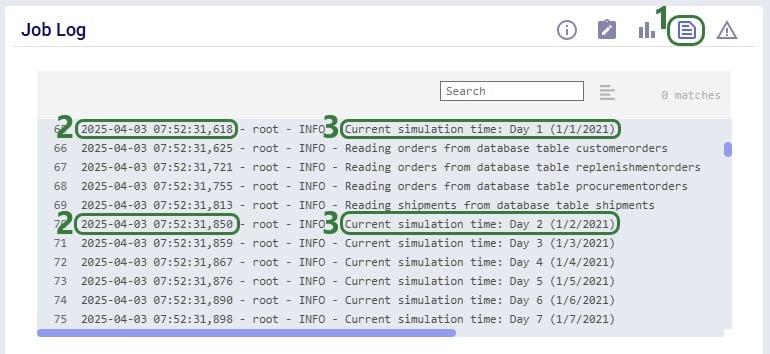
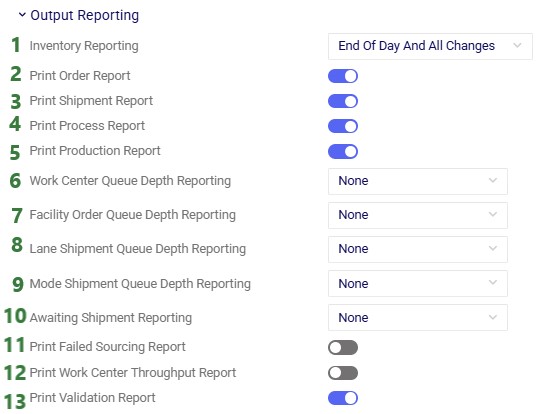
The inventory engine in Cosmic Frog (called Dendro) uses a genetic algorithm to evaluate possible solutions in a successive manner. The parameters that can be set dictate how deep the search space is and how solutions can evolve from one generation to the next. Using the parameter defaults will suffice for most inventory problems, they are however available to change as needed for experienced users.

1. Number Of Generations – the number of generations the genetic algorithm will go through and calculate. The default value is 5.
2. Number Of Genes Per Generation – This is the population size, i.e. the number of candidate solutions maintained in the population throughout the algorithm. The default value is 20.
3. Number Of Offsprings – this specifies how many offsprings are considered from the 2^nd until the last generation. This is the number of new candidate solutions created during a step (generation) of the genetic algorithm. The N best solutions from the current population and these offsprings are kept, where N is the population size parameter (Number Of Genes Per Generation, see previous bullet) and then the algorithm moves on to the next step. The default value is 20.
4. Mutation Probability – the chance that a gene factor will mutate from one generation to the next. The default is 10.
5. Max Values To Mutate – the maximum number of gene factors that are allowed to mutate from one generation to the next. The default value is 5.
6. Crossover Probability – the chance that crossover will occur between genes, e.g. genes are swapped. The default value is 90.
7. Number Of Crossovers – the number of crossover points. The default value is 2.
8. Random Seed – set the seed of the random number generator of the algorithm to start generating the initial population in an area where optimal solutions are likely to be found. When left blank (the default value), the initial population is generated randomly.
9. Fitness Score Calculator – available to enable using a customized approach and class name in the code (Optilogic can provide advice and the options for this). When this is left blank (the default value), the data from the Output Factors input table is used.
10. Automatically Generate Input Factors – automatically populate the Input Factors table before running Dendro. For details on Input Factors, please see the Dendro: Input Factors Guide.
11. Automatically Generate Output Factors – automatically populate the Output Factors table before running Dendro. For details on Output Factors, please see the Dendro: Output Factors Guide.
12. Automatically Run Demand Classification – automatically run the Demand Classification utility before running Dendro to calculate reasonable inventory policy values rather than starting from existing ones. Basic Safety Stock logic is used to determine the initial inventory policy for each facility-product combination.
13. Algorithm Selection – choose which Dendro algorithm to use. Options are:
    1. Genetic Algorithm: Dendro's Genetic Algorithm explores thousands of different inventory policy combinations, simulates each one to see how it performs, and gradually evolves toward the best possible solution. For details on the Genetic Algorithm, please see the Dendro: Genetic Algorithm Guide.
    2. Fast Dendro: A deterministic heuristic that skips the genetic algorithm entirely. Instead of evolving a population, it:
       1. Loads inventory policies and simulation output stats (fill rate, ready rate, etc.)
       2. Iteratively adjusts reorder points up/down using a ratio-based heuristic to hit target service levels
       3. Runs one simulation per iteration (not a full population)
    3. Hybrid: Embeds the Fast Dendro heuristic inside the Genetic Algorithm. Specifically:
       1. Runs the Genetic Algorithm (populations, generations, crossover/mutation)
       2. Instead of running a raw simulation for each candidate, it first applies the Fast Dendro heuristic to warm-start/adjust inventory policies before evaluating fitness
       3. Effect: The Genetic Algorithm explores the policy space at a higher level (e.g., which policies to include/exclude, structural choices), while Fast Dendro handles the fine-tuning of reorder point values within each GA evaluation.
14. Auto-adjust Starting Inventory – when this option is turned on (the default), initial inventory values are automatically adjusted after a Dendro run. Initial inventory will be calculated based on the optimized inventory policies and will be set to S, the order-up-to quantity, for (s,S) policies and to R + Q for (R,Q) policies, where R is the reorder point and Q the reorder quantity.
15. Service Metric – choose which service level metric to optimize against when using the Fast Dendro algorithm (not applicable to the Genetic Algorithm and Hybrid algorithm options). Options are:
    1. Fill Rate: standard fill rate – percentage of customer demand fulfilled immediately from stock
    2. Ready Rate: measures the probability of having no stockouts
    3. Custom Ready Rate: when this option is selected, Dendro will use facility-product ready rates specified on the Inventory Policies Advanced input table instead of a global value.
    4. OTIF: on-time-in-full rate
16. Default Service Target (%) – the default target service/level for facility-product combinations that do not have a specific target specified. This option is used for:
    1. When using the Fast Dendro algorithm if target service is not specified in the Inventory Policies Advanced input table.
    2. When automatically generating Input Factors (bullet 10 above) when using the Genetic Algorithm. The default service target value informs how to set ranges on reorder point.
    3. When automatically generating Output Factors (bullet 11 above) when using the Genetic Algorithm. The default service target value informs how to construct the Service output factor.
    4. When automatically running Demand Classification (bullet 12 above) this default service target is used when performing textbook safety stock calculations.
17. Strictly Enforce Minimum Service – determines policy selection behavior. When turned off (the default), it allows selection of policies which are slightly below the target service level (set by Default Service Target (%), see previous bullet) if they are significantly more cost-efficient. When turned on, the target service level needs to be met or exceeded.
18. Simulation Job Size – users can choose the resource size for the simulation runs that will be done during each generation of the Dendro algorithm. This can be set independently from the resource size that is selected above the Technology Parameters, which is used for the Parent run job of the model run.

Transportation (Hopper) Parameters

1. Run Load Balancing – if weekly demand needs to be balanced over a week, the Load Balancing Demand and Load Balancing Schedules input tables can be used to set this up. If both the Shipments table and the Load Balancing Demand/Schedules tables are populated, by default the Shipments table will be used and the Load Balancing Demand/Schedules tables will be ignored. To switch to using the Load Balancing Demand/Schedules tables (and ignoring the Shipments) table, the Run Load Balancing toggle needs to be switched to on (toggle to the left and grey is off; to the right and blue is on).
2. Solver Focus – controls the solution improvement phase of the solve. Options are:
   1. Normal Mode: uses the standard improvements, usually providing a good balance between finding good solutions and runtime.
   2. Fast Mode: skips the solution improvement phase entirely, providing the fastest runtimes. However, the solutions may be less good as compared to using the other 2 modes.
   3. High Precision Mode: uses a more detailed solution improvement phase. Note that this can lead to longer runtimes.
3. Facility Decomposition – when this option is turned on (the default), the VRP (Vehicle Routing Problem) is split into multiple subproblems, each associated with a specific facility or depot. The solution process is simplified as compared to trying to solve everything simultaneously, leading to shorter runtimes. If the problem can mathematically be entirely decomposed (e.g. when modelling completely independent facilities used for milk run pick-ups) the results will be very close or the same as when the decomposition option is not used. If this option is used for other problems, like for example interleaved models, it can potentially lead to higher cost solutions.
4. Max Run Time In Improvement Phase (Seconds) – use this option if you want to put a limit on the time spent by the algorithm in the solution improvement phase. It is set in seconds, so in order to limit this phase to 10 minutes, you need to set this parameter to a value of 600.
5. Print Detailed Unrouted Shipment Report – when this option is turned on, the Transportation Unrouted Shipment Report output table will be populated. Each record gives an explanation of why a given shipment cannot be inserted into an individual route in the solution. This helps with diagnosis of unrouted shipments, since the reasons might be different for different routes (e.g., capacity exceeded, incompatible time window, breaking of a relationship constraint, etc). The default is off, as the table can get quite large.
6. Complete Service In Time Window – when this option is turned off (the default), any service time needs to start within the business hours of a stop but is not required to complete within the business hours. Similarly, pickup or delivery of shipments needs to start within the pickup / delivery time windows but does not need to be completed within them. When turned on, any service duration does need to be completed within the location's business hours. This also goes for needing to complete deliveries / pickups within the location's delivery / pickup time windows.

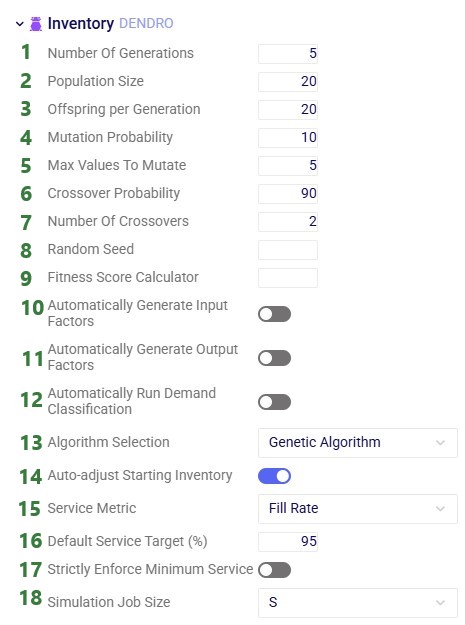
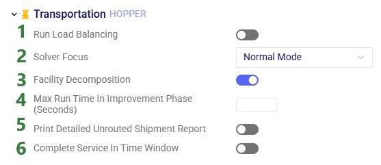
As always, please feel free to contact Optilogic Support at support@optilogic.com in case of questions or feedback.

DataStar users typically will want to use data from a variety of sources in their projects. This data can be in different locations and systems and there are multiple methods available to get the required data into the DataStar application. In this documentation we will describe the main categories of data sources users may want to use and the possible ways of making these available in DataStar for usage.

If you would first like to learn more about DataStar before diving into data integration specifics, please see the Navigation DataStar articles on the Optilogic Help Center.

Overview

The following diagram shows different data sources and the data transfer pathways to make them available for use in DataStar:

1. Local Data – data that is available locally on a DataStar user’s computer, typically Excel workbooks, CSV files, and SQL databases.
2. ‍External Data – data that sits outside of a user’s local computer. This usually falls into one of the following categories: ‍
   
   1. Cloud Storage: examples are Google Sheets, OneDrive, and Amazon S3 ‍
   2. Cloud Data Warehouse: examples are Google Big Query, AWS Amazon Redshift, Snowflake, and Microsoft Azure‍
   3. ERP and Planning Systems: examples are SAP, Kinaxis, Oracle, and Infor

3. Optilogic Platform – data can be stored in the user’s account on the Optilogic platform. The files available in a user’s account can be viewed using the Explorer application. To learn more about the Explorer, please see this Getting Started Help Center article.

4. DataStar – the DataStar application is also hosted on the Optilogic platform, and this is where we want to be able to use the data from the different sources.

5. For local data, the steps to go from the files sitting on the user’s computer to using them in DataStar are as follows (these are explained in more detail in the “Local Data” section below):
   
   1. Upload the files to the Optilogic platform. This can be done one file at a time or multiple files simultaneously, and either manually or programmatically.
      
      • Please note that for local PostgreSQL databases users need to programmatically connect to the database, extract the data and load this data onto the Optilogic platform.
   2. Set up a Data Connection from within DataStar to the files now present in the Explorer so that DataStar can access the files.
   3. Use Import tasks using this created Data Connection as the source to pull data into the DataStar project(s) that need to use this data.

6. For external data, there are 2 main methods that can be used:
   
   1. Utilize ETL tools, automation platforms, or custom scripts to push data onto the Optilogic platform. Here the user starts the process of data extraction and upload to the Optilogic platform from within the tool / platform / script, so it is a “push” action from the customer side. See also the External Data - "Push" from Customer Side section further below for more details.
      
      • Some of these tools can connect to a variety of data sources and extract data in CSV and/or Excel format, such as Talend and Azure Data Factory. These extracted files can then be pushed onto the Optilogic platform by the middleware. Once available there, the steps from bullets 5b and 5c can be taken to make the data available for use in DataStar.
      • Data extracted by the middleware tool can also be landed directly into the Project Sandbox of a DataStar project or in a PostgreSQL database for staging.
   2. Scripts and utilities from the Optilogic platform side can be used to pull data from various sources onto the platform and typically copy the data straight into the Project Sandbox of a DataStar project. These scripts can exist and be run 1) locally on a user’s computer, or 2) on the Optilogic platform in the user’s account (outside of DataStar), or 3) from inside DataStar leveraging Run Python and Run Utility tasks. Several template scripts and utilities are available currently in the Resource Library application on the Optilogic platform; for more details, see the External Data - "Pull" from Optilogic Side section further below.

Local Data

We will dive a bit deeper into making local data available for use in DataStar building upon what was covered under bullets 5a-5c in the previous screenshot. First, we will familiarize ourselves with the layout of the Optilogic platform:

1. Access your account on the Optilogic platform by logging into it from optilogic.app or cosmicfrog.com.
2. Once logged in, the breadcrumb trail in the toolbar at the top will always indicate where in the platform you are working currently. The format is: Organization (always Optilogic) – Team (if working in a Team workspace, otherwise not shown when working in your own account) – Application (Home here) – Project / Model / File name (only shown if anything is open in the currently open application).
3. When first logging in, you will land on the Home page of the platform where you can get started with videos, training courses, links to useful resources and read the latest Optilogic news.
4. On the left-hand side the list of applications available on the platform is shown. Most users will be mainly using Cosmic Frog and/or DataStar for their supply chain modelling and data workflow purposes, using the other applications to support the use of these 2 main applications.
5. The other applications can also be accessed from the list. Note that the order of the applications may be different in your account. You can drag and drop the application icons to re-arrange the order. In case not all applications are shown in the list, you can click on the icon with 3 horizontal dots to show all applications.
6. The Explorer sits across all applications on the platform. It can be opened and closed by clicking on the chevron icon at the left top. When open:
   
   1. The folders present in the user’s account are shown. These can be expanded by clicking on the chevron icons to the left of the folder names.
   2. Quick search, filter, share, zoom to file, collapse all, and refresh options are available to help the user find their file(s) of interest quickly.

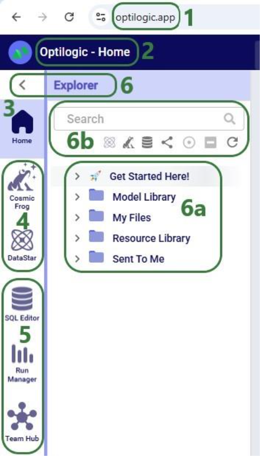
Next, we will cover the 3 steps to go from data sitting on a user’s computer locally to being able to use it in DataStar in detail through the next set of screenshots. At a high-level the steps are:

1. Upload files to the Optilogic platform.
2. Create Data Connections to these files from within DataStar.
3. Create Import tasks in the DataStar project(s) using the Data Connections as the data source.

Upload Data to Optilogic Platform

To get local data onto the Opitlogic platform, we can use the file / folder upload option:

1. Open the Explorer if not yet open by clicking on the chevron icon at the top left.
2. Right-click on the folder you want to upload files to.
3. Select Upload Files from the context menu. The following form comes up:

1. The folder that was right clicked on will be the one the files will be uploaded to.
2. If wanting to upload 1 or a few files from one folder, choose the Add Files option.
3. If wanting to upload all or almost all files from one folder, choose the Add Folder option.

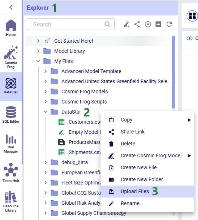
Select either the file(s) or folder you want to upload by browsing to it/them. After clicking on Open, the File Upload form will be shown again:

1. You can go back and re-select what you want to upload by using the Add Files or Add Folder buttons.
2. A summary and list of the files to be uploaded is displayed.
3. Two of the files have a warning and are highlighted in yellow, this is because files of the same name already exist in the folder we are about to upload these files into. One option is to rename the file so there is no naming conflict; click on the Rename icon to do so.
4. Instead of renaming a file with a conflicting name, it can also be removed from the list so it will not be uploaded.
5. Another option to resolve file name conflicts is to allow overwriting of already existing files with files of the same name that are going to be uploaded. Switch the option to on if overwriting is allowed. If not allowed, then any name conflicts will need to be resolved before the upload can start.
6. Once files have been selected and any naming conflicts have been resolved (when overwriting is not allowed), the Upload button can be used to start the upload of the file(s).
7. If at any point the user decides they do not want to go ahead with uploading any files, they can click on the Cancel button.

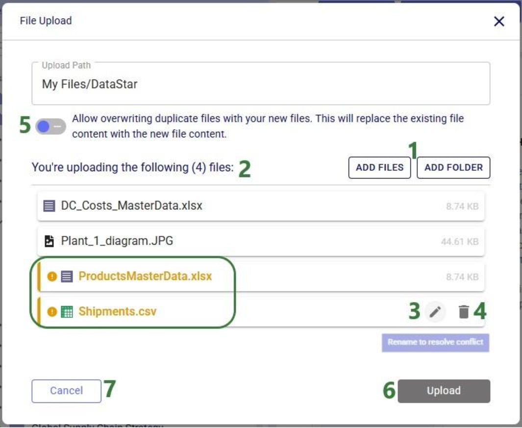
Note that files in the upload list that will not cause name conflicts can also be renamed or removed from the list if so desired. This can for example be convenient when wanting to upload most files in a folder, except for a select few. In that case use the Add Folder option and in the list that will be shown, remove the few that should not be uploaded rather than using Add Files and then manually selecting almost all files in a folder.

Once the files are uploaded, you will be able to see them in the Explorer by expanding the folder they were uploaded to or searching for (part of) their name using the Search box.

Create Data Connections

The second step is to then make these files visible to DataStar by setting up Data Connections to them:

1. Within DataStar (open it by clicking on the DataStar application icon in the list of applications on the left), click on the Create Data Connection button.
2. Give the connection a name and optionally a description, then choose the connection type.  
3. The connection type options are currently: CSV files, Excel Files (beta version), Cosmic Frog models, or PostgreSQL databases.
   
   1. Note that currently only connections to PostgreSQL databases which are hosted on the Optilogic platform can be created.  

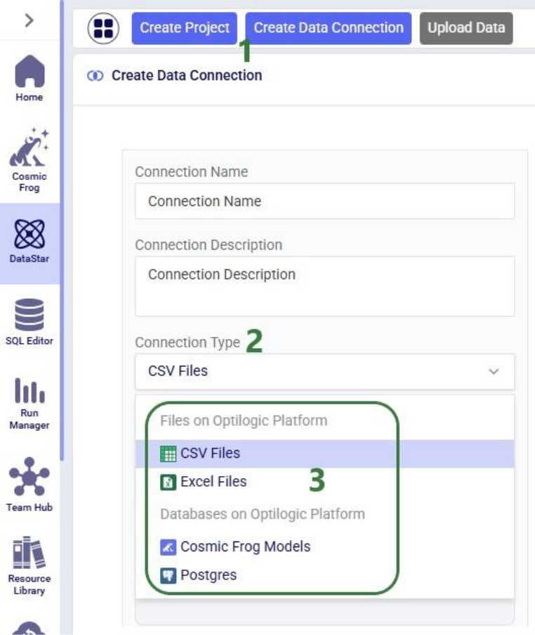
After setting up a Data Connection to a Cosmic Frog model and to a CSV file, we can see the source files in the Explorer, and the Data Connections pointing to these in DataStar side-by-side:

1. DataStar is the active application as indicated by its icon having a darker background.
2. DataStar will be shown in the center part of the platform. On the DataStar start page, the Data Connections tab is open.
3. The Explorer is also open and is shown on the left-hand side.
4. The source for the connection named “Empty CF model for DataStar Export” (connection type = Cosmic Frog) is the model named “Empty Model for DataStar.frog”, shown in the /My Files/DataStar folder in the Explorer. DataStar can now access this model.
5. Similarly, the source for the connection named “Historical Shipments” (connection type = CSV) is the file named Shipments.csv shown in the /My Files/DataStar folder in the Explorer. DataStar can now access this file too.

Import Data into DataStar Projects

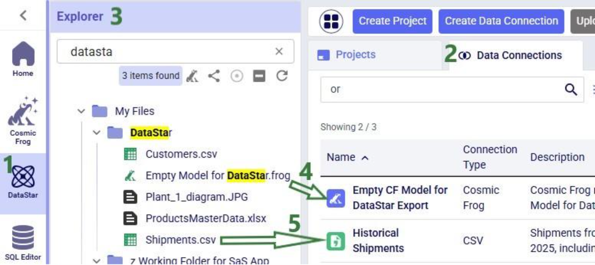
To start using the data in DataStar, we need to take the third step of importing the data from the data connections into a project. Typically, the data will be imported into the Project Sandbox, but this could also be into another Postgres database, including a Cosmic Frog model. Importing data is done using Import tasks; the Configuration tab of one is shown in this next screenshot:  

1. The type of task we are configuring is Import.
2. First, the Source Data Connection will be configured, this is the data source from which data will be pulled into DataStar.
3. We can select the Source Data Connection from the drop-down list showing all Data Connections that have been set up (Excel, CSV, Cosmic Frog model or other Postgres database). In the screenshot we are showing the Cosmic Frog model connection and CSV file connection of which we showed the data connections and the files they point to in the previous screenshot.
4. Next, the Target Data Connection for the import is specified, here a new table named “Shipments_2025” in the Project Sandbox.

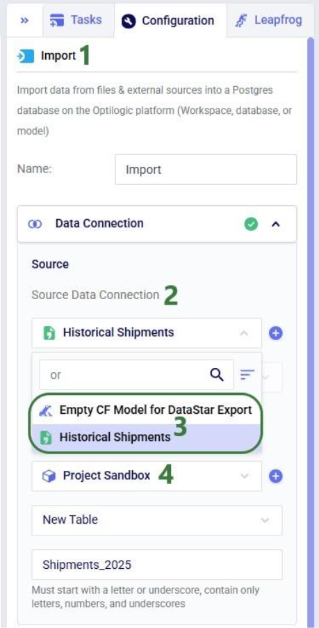
The 3 steps described above are summarized in the following sequence of screenshots:

Local Data Refresh

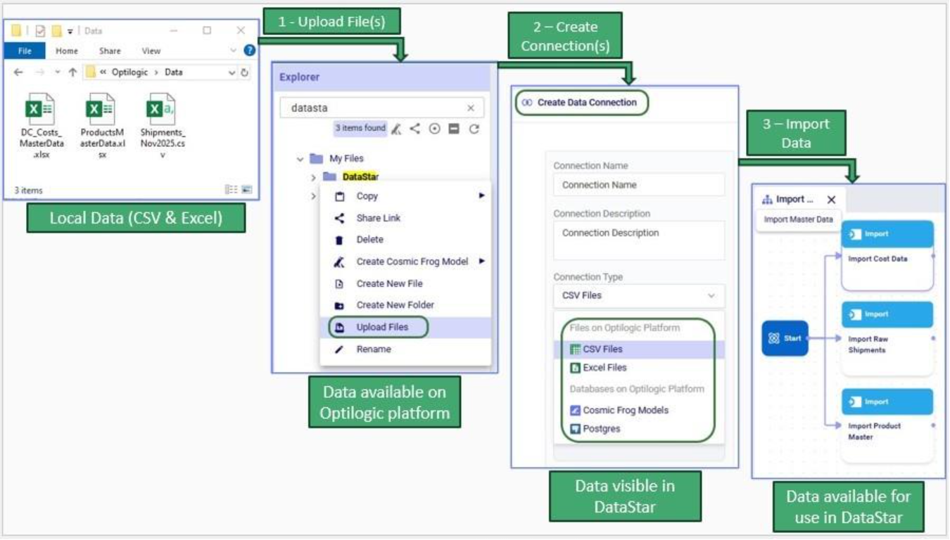
For a data workflow that is used repeatedly and needs to be re-run using the latest data regularly, users do not need to go through all 3 steps above of uploading data, creating/re-configuring data connections, and creating/re-configuring Import tasks to refresh local data. If the new files to be used have the same name and same data structure as the current ones, replacing the files on the Optilogic platform with the newer ones will suffice (so only step 1 is needed); the data connections and Import tasks do not need to be updated or re-configured. Users can do this manually or programmatically:

1. Manual local data refresh: as described above by using the upload files / folder option from within the Explorer. Note that the user will need to take care of archiving any previously used files themselves in case this is required. Users can choose to do this either on the Optilogic platform or locally. When archiving on the platform, a quick manual way can be to rename the folder with the outdated files, create a new folder with the same name as the old folder had prior to renaming, upload the required files into this new folder (note that this only works well if replacing all files with newer ones). ‍
2. Programmatic local data refresh: users can use scripts to bulk upload their local files into the desired folder in their Optilogic account or load data from local files straight into a Postgres database (which could be a project sandbox). A Python utility that can be leveraged as-is or used as a starting point to modify to users’ needs is available from the Resource Library:
   
   1. A Python utility which imports local CSV-files straight into a Postgres database on the Optilogic platform is available here on the Resource Library. The utility and its detailed documentation can be downloaded / copied from the Resource Library. This utility has the option of appending uploads to existing tables instead of creating a new table for each CSV file and it is designed for high-speed ingestion while maintaining data integrity and reproducibility.
   2. A Python Script for bulk uploading local files to the Optilogic platform with an auto-archive option built in can be found here on the Resource Library. The script and its detailed documentation can be downloaded / copied from the Resource Library. In a nutshell, the script:
      
      • Requires the user to specify the local folder containing the files to be uploaded and the target folder on the Optilogic platform to upload the files to.
      • Users can configure the script further to their needs with a few user-defined settings:
        
        • Choose to upload all files, only the CSV and Excel files, or a user-defined list of files from the upload folder.
        • Option to auto-archive files that would give naming conflicts due to having the same name into a different folder prior to overwriting them. By default, the folder to archive files to will have the name of the target folder suffixed with the date; this can be overridden with a user-defined suffix.

External Data - “Push” from Customer Side

This section describes how to bring external data into DataStar using supported integration patterns where the data transfer is started from an external system, e.g. the data is “pushed” onto the Optilogic platform.

Integrating Data Using Optilogic APIs

External systems such as ETL tools, automation platforms, or custom scripts can load data into DataStar through the Optilogic Pioneer API (please see the Optilogic REST API documentation for details). This approach is ideal when you want to programmatically upload files, refresh datasets, or orchestrate transformations without connecting directly to the underlying database.

Key points:

1. The API uses standard Optilogic authentication
2. External tools simply perform authenticated API calls
3. The same endpoints used by DataStar’s native Python utilities are available for external integrations

Please note that Optilogic has developed a Python library to facilitate scripting for DataStar. If your external system is Python based, you can leverage this library as a wrapper for the API. For more details on working with the library and a code example of accessing a DataStar project’s sandbox, see this “Using the DataStar Python Library” help center article. 

Integrating Data Using Direct Database Connections

Every DataStar project is backed by a PostgreSQL database. You can connect directly to this database using any PostgreSQL-compatible driver, including:

1. ODBC
2. JDBC
3. Native PostgreSQL clients
4. Cloud integration connectors
5. BI tools or data pipelines that support Postgres connections

This enables you to write or update data using SQL, query the sandbox tables, or automate recurring loads. The same approach applies to both DataStar projects and Cosmic Frog models since both use PostgreSQL under the hood. Please see this help center article on how to retrieve connection strings for Cosmic Frog model and DataStar project databases; these will need to be passed into the database connection to gain access to the model / project database.

External Data - “Pull” from Optilogic Side

Template Scripts and Utilities

Several scripts and utilities to connect to common external data sources, including Databricks, Google Big Query, Google Drive, and Snowflake, are available on Optilogic’s Resource Library:

1. Go to the Resource Library application while logged in on the Optilogic platform.
2. Click on the DataStar button at the right top to filter the list of resources for those specific to DataStar.
3. Optionally, use the Tags drop-down to filter the list further down to find what you are looking for quickly. Here we have selected 2 tags: "Extensibility Tool" and "Utility".
4. Browse the list and click on a resource of interest to select it, here we clicked on the "Google Big Query Insert Script" resource.
5. After clicking on it, a description of the resource appears on the right hand-side.
6. Associated files can be downloaded by using these Download buttons. Each contains a user guide which describes the script / utility and lets users know what they need to configure in them to start using them.
7. The blue buttons at the right bottom can be used to gain access to this resource. Click on the Copy to Account button to start using the resource on the Optilogic platform. Scripts can for example be viewed, edited, and run in the Lightning Editor application. The Download All option can be used if you want to use the available files locally.

These utilities and scripts can function as a starting point to modify into your own desired script for connecting to and retrieving data from a certain data source. You will need to update authentication and connection information in the scripts and configure the user settings to your needs. For example, this is the User Input section of the “Databricks Data Import Script”:

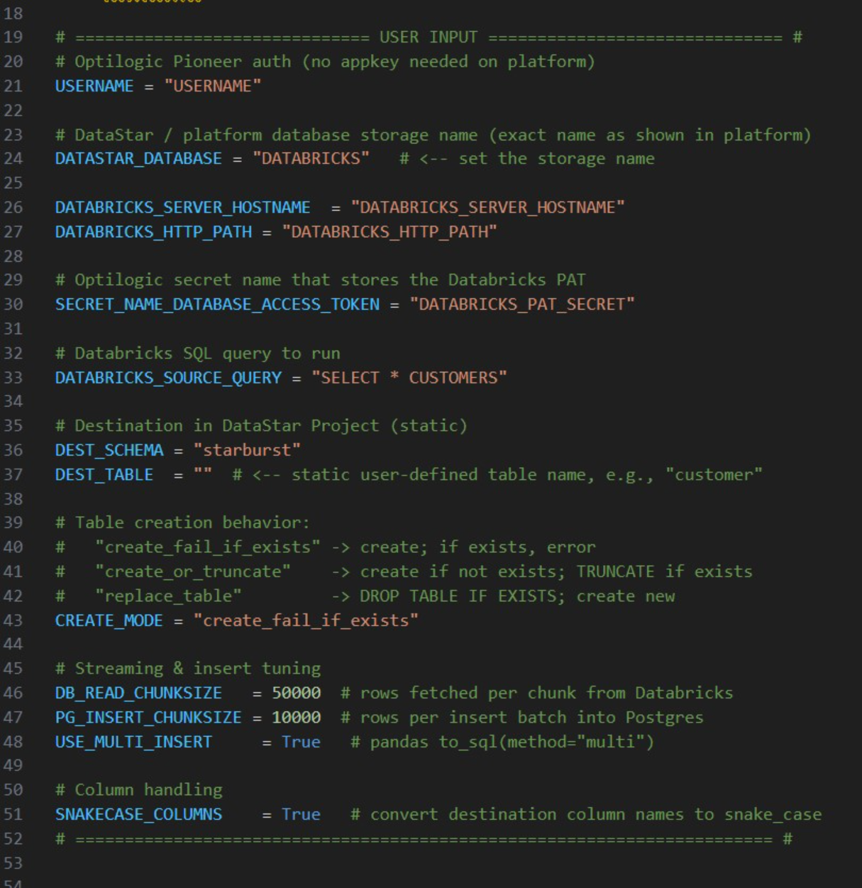
The user needs to update following lines; others can be left at defaults and only updated if desired/required:

• Line 21: update “USERNAME” to the user’s own username
• Line 24: update “DATABRICKS” to the name of the DataStar project to import the databricks data into
• Line 26 and 27: update the “DATABRICKS_SERVER_HOSTNAME” and “DATABRICKS_HTTP_PATH” to the hostname and path of the user’s Databricks instance
• Line 30: update “DATABRICKS_PAT_SECRET” to the user’s Databricks Personal Access Token (PAT) to ensure authenticated access to Databricks
• Line 33: update the query to run to extract data from Databricks. This example “SELECT * FROM CUSTOMERS” retrieves all records with all columns from a table named CUSTOMERS
• Line 37: update this to the name of the destination table in the DataStar project database

Before you Start

1. We highly recommend taking some extra time up-front to think through naming conventions of folders (local and on the Optilogic platform), files, and data connections in DataStar before creating workflows that are meant to be repeatable and will need regular data refreshes. Deciding on this beforehand can save a lot of time further down the road.
2. It is also recommended to think through beforehand how much data transformation and filtering is done as part of the data pull/push process. Our guidance here is as follows:
   
   1. Send raw data onto the Optilogic platform when you want maximum transparency, easier debugging, lineage visibility, and the flexibility to iterate or adjust logic downstream.
   2. Transform data upstream when you know you only need a curated subset, want to reduce noise, or are optimizing for performance, cost, or simplicity.

For any questions or feedback, please feel free to reach out to the Optilogic support team on support@optilogic.com.

In this quick start guide we will show how Leapfrog AI can be used in DataStar to generate tasks from natural language prompts, no coding necessary!

Using Leapfrog to create a Run SQL task

This quick start guide builds upon the previous one where a CSV file was imported into the Project Sandbox, please follow the steps in there first if you want to follow along with the steps in this quick start. The starting point for this quick start is therefore a project named Import Historical Shipments that has a Historical Shipments data connection of type = CSV, and a table in the Project Sandbox named rawshipments, which contains 42,656 records.

The Shipments.csv file that was imported into the rawshipments table has following data structure (showing 5 of the 42,656 records):

Our goal in this quick start is to create a task using Leapfrog that will use this data (from the rawshipments table in the Project Sandbox) to create a list of unique customers, where the destination stores function as the customers. Ultimately, this list of customers will be used to populate the Customers input table of a Cosmic Frog model. A few things to consider when formulating the prompt are:

• Leapfrog will not know what data to use to generate the customer list from unless we tell it, so we need to indicate in our prompt that the rawshipments table is to be used for this task. We can use the @ character to bring up a list of tables present in the project sandbox.
• We may need to tell Leapfrog which column to use to create customers from, as there is no customer name (or similar) column in this data. We want it to use the Destination Store column to create the customers from. Again, we can use the @ character: after selecting a table from the list of tables in the sandbox, we can also access a list of column names present in the selected table.
• Each Destination Store has multiple records in this file, since it is transactional data over a period of time (June 1, 2024 – July 31, 2025) where stores placed and received multiple orders and each was also served by multiple DCs. Therefore, if we want the customer list to include location information, which is contained in the destination latitude and destination longitude columns, we need to think about if we want Leapfrog to do anything with these columns as there is a chance these are not all exactly the same for all records with the same Destination Store. We will tell Leapfrog to take the average of the destination latitude and destination longitude to come up with the coordinates of each unique customer.
• The data contains shipments for 14 months, but we only want to use the records of the 12 months starting from July 1, 2024. We will need to tell Leapfrog this.
• Leapfrog is aware of the Anura database schema which is what Cosmic Frog models use underneath. We can therefore reference this in prompts so that tables generated using tasks created by Leapfrog match this schema.

Within the Import Historical Shipments DataStar project, click on the Import Shipments macro to open it in the macro canvas, you should see the Start and Import Raw Shipments tasks on the canvas. Then open Leapfrog by clicking on the Ask Leapfrog AI button to the right in the toolbar at the top of DataStar. This will open the Leapfrog tab where a welcome message will be shown. Next, we can write our prompt in the “Write a message…” textbox.

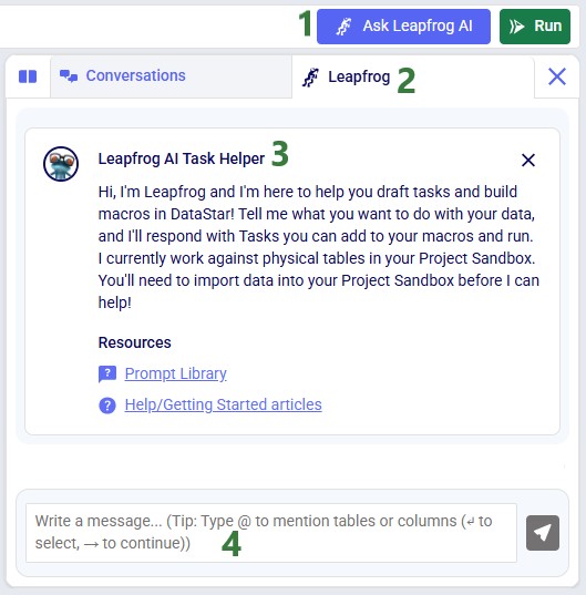
Keeping in mind the 5 items mentioned above, the prompt we use is the following: “Use the @rawshipments table to create unique customers (use the @rawshipments.destination_store column); average the latitudes and longitudes. Only use records with the @rawshipments.ship_date between July 1 2024 and June 30 2025. Match to the anura schema of the Customers table”. Please note that:

• Tips for writing successful prompts and variations of this prompt (some working, others not) can be found in the Tips for Prompt Writing section further below.
• The use of the @ character to quickly find sandbox tables and their columns is explained in more detail in the Leapfrog section of the Getting Started with DataStar help center article.

After clicking on the send icon to submit the prompt, Leapfrog will take a few seconds to consider the prompt and formulate a response. The response will look similar to the following screenshot, where we see from top to bottom:

• The prompt
• Leapfrog’s text response about what it did in the Documentation section
• The type of task it has created, here a Run SQL one
• The target data connection will always be the Project Sandbox for Leapfrog generated tasks
• Then follows the SQL script that was generated to perform the actions user asked for in the prompt.
• A Notes section repeating the text from the Documentation part of the response, with an indication of how long the response took to generate and the number of words and characters added. This section will be added as a Notes section if a task is created and added to the macro from the Leapfrog response.
• Users can optionally give a thumbs up or down to give feedback on the Leapfrog response which can be used to improve the Leapfrog algorithm.
• The Add Macro button can be used to add the propsed Run SQL task to the macro.

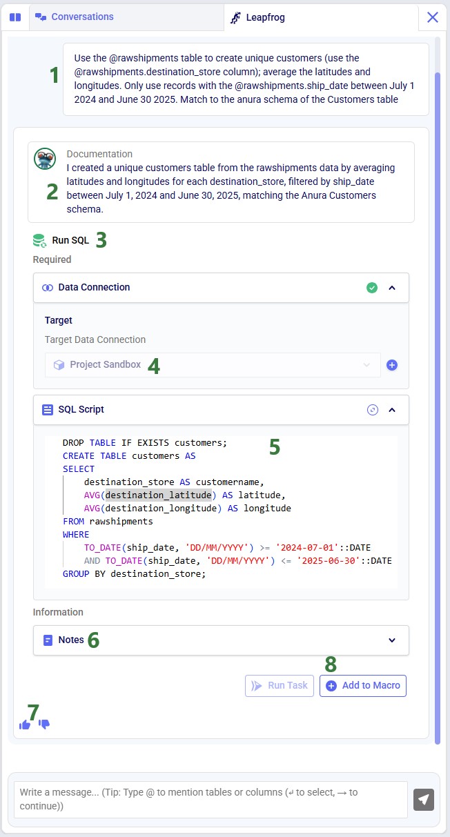
For copy-pasting purposes, the resulting SQL Script is repeated here:

DROP TABLE IF EXISTS customers;
CREATE TABLE customers AS 
SELECT 
  destination_store AS customername, 
  AVG(destination_latitude) AS latitude, 
  AVG(destination_longitude) AS longitude 
FROM rawshipments 
WHERE
  TO_DATE(ship_date, 'DD/MM/YYYY') >= '2024-07-01'::DATE
  AND TO_DATE(ship_date, 'DD/MM/YYYY') <= '2025-06-30'::DATE
GROUP BY destination_store;

‍

Those who are familiar with SQL, will be able to tell that this will indeed achieve our goal. Since that is the case, we can click on the Add to Macro button at the bottom of Leapfrog’s response to add this as a Run SQL task to our Import Shipments macro. When hovering over this button, you will see Leapfrog suggests where to put it on the macro canvas and to connect it to the Import Raw Shipments task, which is what we want. When next clicking on the Add to Macro button it will be added.

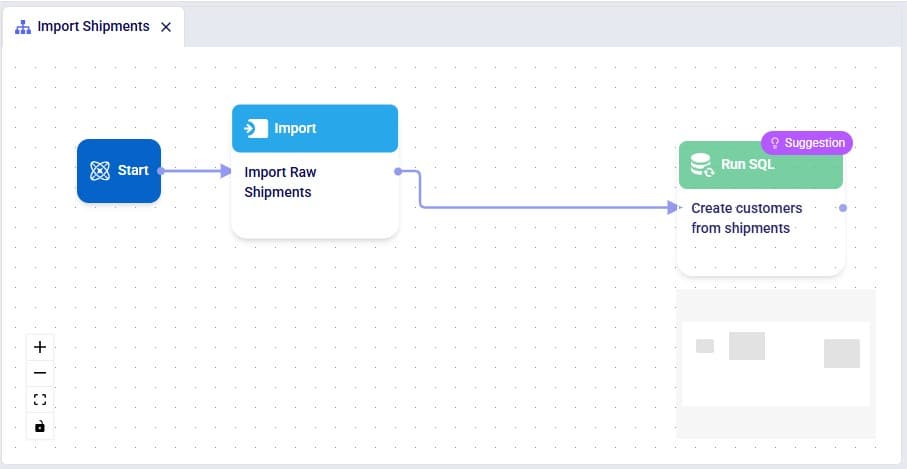
We can test our macro so far, by clicking on the green Run button at the right top of DataStar. Please note that:

• For the moment, you will need to have run the "Import Raw Shipments" task before being able to reference the rawshipments table it creates in the Project Sandbox. In other words, before submitting the prompt in Leapfrog, the "Import Raw Shipments" task needs to have been run.
• Similarly, when building upon this new "Create customers from shipments" task (for example to take the resulting customers and import them into the Customers table of a Cosmic Frog model), it is also needed to run this task before it can be referenced in subsequent tasks. This will not be necessary anymore in future updates to DataStar.

Once the macro is done running, we can check the results. Go to the Data Connections tab, expand the Project Sandbox connection and click on the customers table to open it in the central part of DataStar:

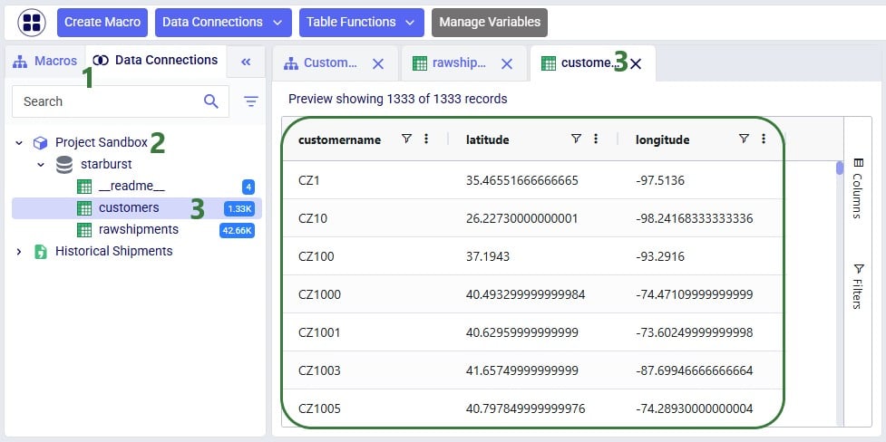
We see that the customers table resulting from running the Leapfrog-created Run SQL task contains 1,333 records. Also notice that its schema matches that of the Customers table of Cosmic Frog models, which includes columns named customername, latitude, and longitude.

Tips for Prompt Writing

Writing prompts for Leapfrog that will create successful responses (e.g. the SQL Script generated will achieve what the prompt-writer intended) may take a bit of practice. This Mastering Leapfrog for SQL Use Cases: How to write Prompts that get Results post on the Frogger Pond community portal has some great advice which applies to Leapfrog in DataStar too. It is highly recommended to give it a read; the main points of advice follow here too:

1. Start with your goal: what do you want the task to accomplish?
2. Mention key elements/dimensions: products, locations, time frames, etc.
3. Name the table(s) and columns: leverage the @character to find the intended table and column names Leapfrog should use
4. Leverage Anura schema knowledge: use text like “match to the anura schema for X table” to create tables in the Cosmic Frog model data format
5. Chain your prompts: ask follow-ups to refine the query (e.g. “like that, but with X changed”, “like that, and with Y added”).
6. Break down complex prompts: if your goal has multiple parts (e.g. filtering, grouping, joining), split it into smaller steps.
7. Reset if needed: if Leapfrog gets off track and follow-up redirections do not work, starting a new conversation can help it reset context and produce better results.

As an example, let us look at variations of the prompt we used in this quick start guide, to gauge the level of granularity needed for a successful response. In this table, the prompts are listed from least to most granular:

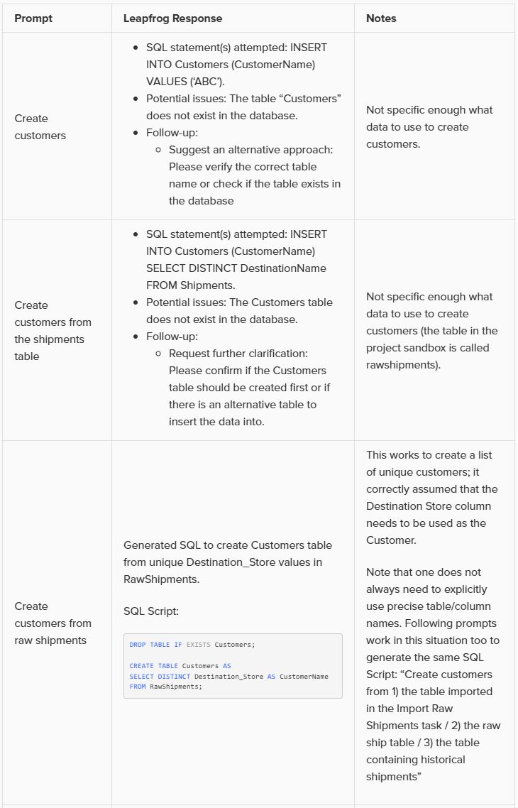
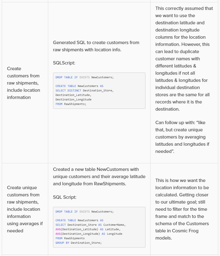
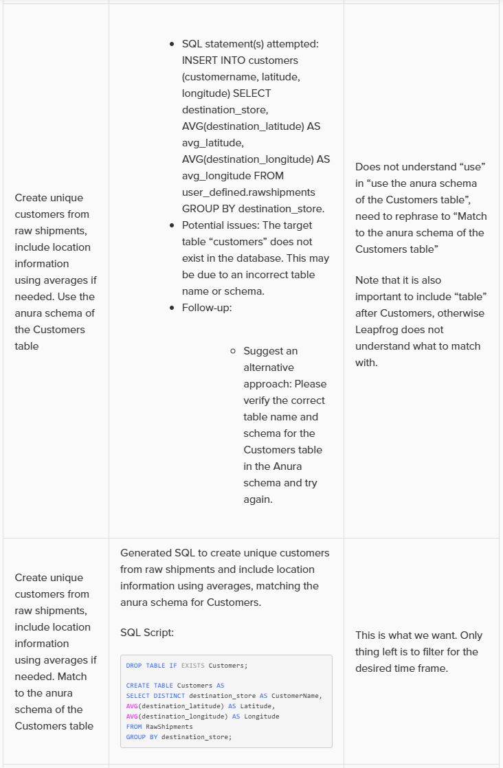
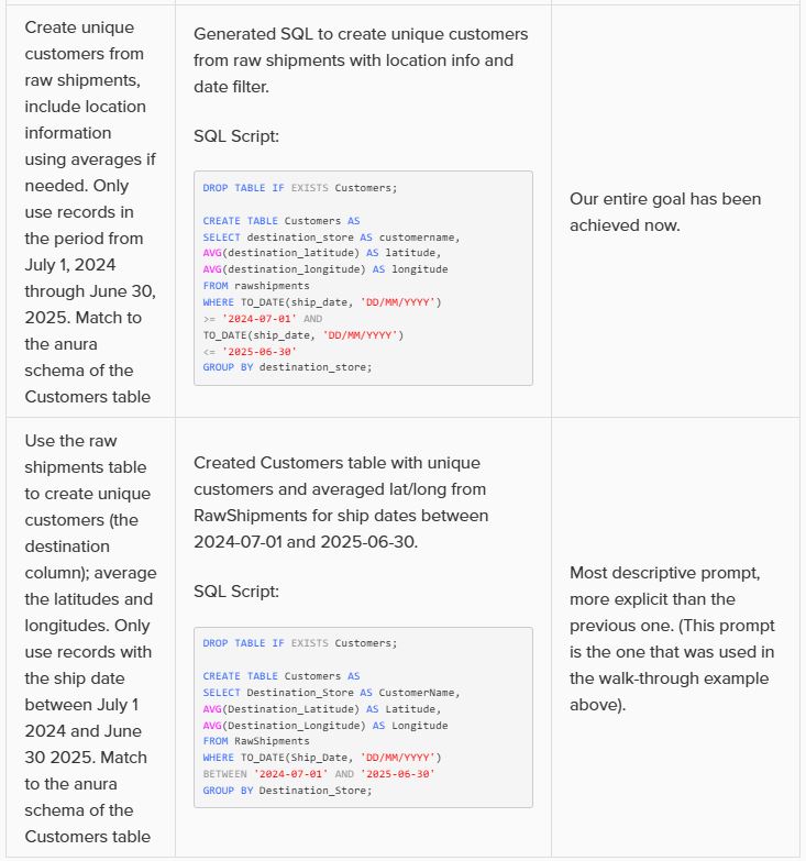
Note that in the above prompts, we are quite precise about table and column names and no typos are made by the prompt writer. However, Leapfrog can generally manage well with typos and often also pick up table and column names when not explicitly used in the prompt. So while generally being more explicit results in higher accuracy, it is not necessary to always be extremely explicit and we just recommend to be as explicit as you can be.

In addition, these example prompts do not use the @ character to specify tables and columns to use, but they could to facilitate prompt writing further.

Helpful Resources

• The Leapfrog Prompt Library on the Frogger Pond community portal.
• All available DataStar documentation on Optilogic's Help Center can be found here in the "Navigating DataStar" section.
  
  • Specific on Leapfrog, see this Leapfrog section in the Getting Started with DataStar article.
• DataStar specific resources such as scripts for uploading data and connecting to external data sources, and template projects can be found on the Resource Library. To filter for DataStar related resources, click on the DataStar button at the top right.

‍

In this quick start guide we will walk through the steps of exporting data from a table in the Project Sandbox to a table in a Cosmic Frog model.

Initial Setup and Quick Start Steps

This quick start guide builds upon a previous one where unique customers were created from historical shipments using a Leapfrog-generated Run SQL task. Please follow the steps in that quick start guide first if you want to follow along with the steps in this one. The starting point for this quick start is therefore a project named Import Historical Shipments, which contains a macro called Import Shipments. This macro has an Import task and a Run SQL task. The project has a Historical Shipments data connection of type = CSV, and the Project Sandbox contains 2 tables named rawshipments (42,656 records) and customers (1,333 records).

The steps we will walk through in this quick start guide are:

1. Create an empty Cosmic Frog model.
2. Set up a data connection to the empty Cosmic Frog model.
3. Add and configure an Export task.
4. Check the results of the complete macro.

Create an empty Cosmic Frog Model

First, we will create a new Cosmic Frog model which does not have any data in it. We want to use this model to receive the data we export from the Project Sandbox.

As shown with the numbered steps in the screenshot below: while on the start page of Cosmic Frog, click on the Create Model button at the top of the screen. In the Create Frog Model form that comes up, type the model name, optionally add a description, and select the Empty Model option. Click on the Create Model button to complete the creation of the new model:

Create Cosmic Frog Model Data Connection

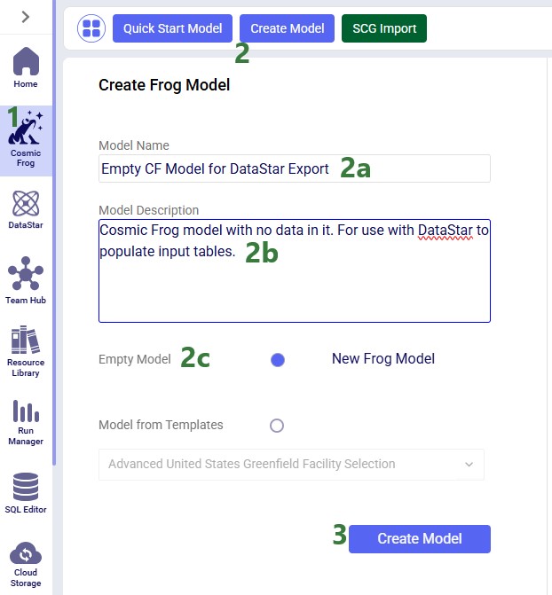
Next, we want to create a connection to the just created empty Cosmic Frog model in DataStar. To do so: open your DataStar application, then click on the Create Data Connection button at the top of the screen. In the Create Data Connection form that comes up, type the name of the connection (we are using the same name as the model, i.e. “Empty CF Model for DataStar Export”),optionally add a description, select Cosmic Frog Models in the Connection Type drop-down list, click on the name of the newly created empty model in the list of models, and click on Add Connection. The new data connection will now be shown in the list of connections on the Data Connections tab (shown in list format here):

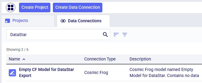
Now, go to the Projects tab, and click on the “Import Historical Shipments” project to open it. We will first have a look at the Project Sandbox and the empty Cosmic Frog model connections, so click on the Data Connections tab:

1. We have opened the Data Connections tab.
2. The Project Sandbox connection has been expanded.
3. We see that the customers table in the Project Sandbox contains 1.33k records. This was the result of creating unique customers from historical shipment data in the previous quick start guide.
4. The empty Cosmic Frog model connection has been expanded too.
5. Scrolling down the list of tables in the model, we see that the customers table has 0 records.

Add Export Task

The next step is to add and configure an Export Task to the Import Shipments macro. Click on the Macros tab in the panel on the left-hand side, and then on the Import Shipments macro to open it. Click on the Export task in the Tasks panel on the right-hand side and drag it onto the Macro Canvas. If you drag it close to the Run SQL task, it will automatically connect to it once you drop the Export task:

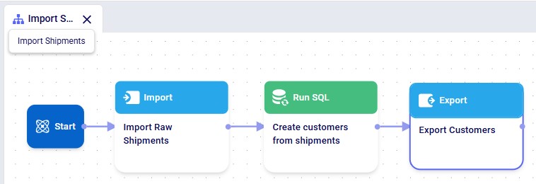
The Configuration panel on the right has now become the active panel:

1. We give the task the name of “Export Customers”.
2. In the Data Connection section, we will configure the source and destination of the export, starting with the source:
   
   1. Select the Project Sandbox as the Data Connection to export from. Clicking on the plus icon to the right allows users to create a new data connection from within the task configuration.
   2. From the table drop-down, select the customers table. A preview of the table can be opened by clicking on the grid icon to the right.
3. It is possible to either export to a Data Connection or export as a .CSV file. We choose the first option.
4. Now we need to configure the destination of the export:
   
   1. In the drop-down list of Data Connections, select the “Empty CF Model for DataStar Export” connection to export into. Again, we can create a new data connection from within this configuration by clicking on the plus icon to the right.
   2. It is possible for the exported data to be added to either a new or an existing table. Select the Existing Table option from the drop-down list.
   3. Now we can click on the Tables drop-down list and scroll to the customers table; select it so it will receive the exported data. Here we can also show a preview of the data in this table by clicking on the grid icon on the right-hand side.
   4. We can choose between Replace, which will overwrite any existing data already present in the table, and Upsert, which will append new data and update any already existing data. We choose the Replace option.
5. In the Data Mapping section, we need to indicate which source column’s data will be exported into which destination column.
   
   1. On the left-hand side, the source column names and their data types are listed.
   2. On the right-hand side, we need to indicate which destination column the source column should export into. We could go through and select the desired column from the drop-down list of all columns in the destination data connection, but we will first give the AutoMap option a try, see the next bullet and screenshot. More details on manually mapping can be found in the Data Mapping Details section further below. Note that there is also a Type column to the right of the Destination Column column, which is not shown in this screenshot.
   3. The AutoMap button can be used to automatically map source columns to destination columns. This is done based on matching column names.

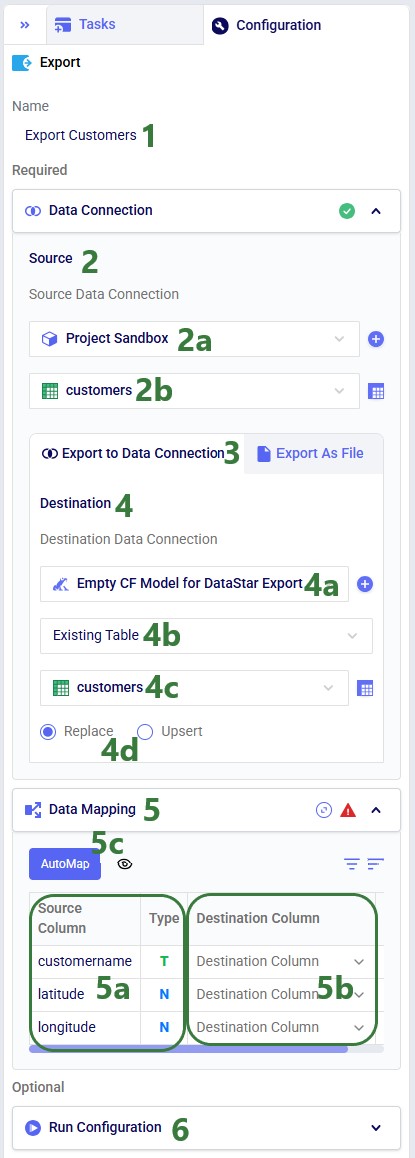
Click on the AutoMap button, and in the message that comes up, select either Replace Mappings or Add New Mappings. Since we have not mapped anything yet, the result will be the same in this case. After using the AutoMap option, the mapping looks as follows:

We see that each source column is now mapped to a destination column of the same name. This is what we expect, since in the previous quick start guide, we made sure to tell Leapfrog when generating the Run SQL task for creating unique customers to match the schema of the customers table in Cosmic Frog models (“the Anura schema”).

Check the Results

If the Import Shipments macro has been run previously, we can just run the new Export Customers task by itself (hover over the task in the Macro Canvas and click on the play button that comes up), otherwise we can choose to run the full macro by clicking on the green Run button at the right top. Once completed, click on the Data Connections tab to check the results:

1. Expand the Empty CF Model for DataStar Export connection and scroll down to the customers table: it now contains 1.33krecords. Click on it to open it in the central part of DataStar.
2. The customers table is now open.
3. We can review that each customer is present and has its latitude and longitude columns populated (they were moved left for the screenshot; you may need to scroll right to see them).

Data Mapping Details

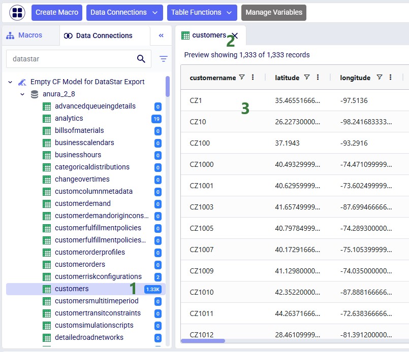
Above, the AutoMap functionality was used to map all 3 source columns to the correct destination columns. Here, we will go into some more detail on manually mapping and additional options users have to quickly sort and filter the list of mappings.

1. To map a Source Column, click on the corresponding field in the Destination Column column, and a drop-down with the list of columns present in the destination data connection will come up.
2. To quickly find a column in the list, use the Search box by typing text in it. Columns with the typed text in their names will be filtered out and shown only.
3. The destination columns can also be filtered by type. Click on the filter icon and check the checkbox(es) of the data types that should be filtered out. The available data types to select from are: Boolean, Date Time, Number, and Text. Note that each data type can be recognized by its first letter abbreviation and distinct font color. These are used in the Type columns and also next to the column names in the drop-down list. For the text data type it is a green T, for number a blue N, etc.
4. If the currently selected field has already been mapped, then it will be highlighted in the drop-down list of column names in the destination data connection. Here, customername is highlighted as this is the current mapping of this field.
5. If the currently selected field has already been mapped, an option to remove the mapping is present at the bottom of the drop-down list. Select this “Remove Selection” option to undo the current mapping.
6. If columns in the destination data connection have already been mapped to a different source column, they will be greyed out in the drop-down list. They cannot be selected. When hovering over these, hover text telling the user which source column this destination column is mapped to comes up.
7. Click on the eye icon to only show the source columns that have been mapped. Unmapped columns will be hidden. This can be convenient when mapping a select subset of many columns: when you think you have mapped all the needed columns, use this to only show the mapped columns and double-check they are all there. Clicking on the icon again will show all source columns again.
8. The list of mappings can also be filtered based on the data type of the source columns. Click on this icon to bring up the checkboxes to check/uncheck the data types that should be shown. The available data types to select from are: Boolean, Date Time, Number, and Text.
9. The list of mappings can be sorted. Click on this icon and choose one of the following three sort options:
   
   1. Source Table Order: orders the mappings based on the sequence of the source columns in the source table.
   2. Name (A-Z): orders the mappings in alphabetical order of the source column names.
   3. Type: orders the mappings in alphabetical order of the source column types, e.g. all Boolean columns first, then all Date Time columns, etc.
10. You can expand the Data Mapping section by clicking on this maximize icon. This allows users to manually map their data in a bigger window.

Helpful Resources

• All available DataStar Help Center articles can be found here: Navigating DataStar.
• DataStar specific resources such as scripts for uploading data and connecting to external data sources, and template projects can be found on the Resource Library. To filter for DataStar related resources, click on the DataStar button at the top right.