In this quick start guide we will walk through the steps of modifying data in a table in the Project Sandbox using Update tasks. These changes can either be made to all records in a table or a subset based on a filtering condition. Any PostgreSQL function can be used when configuring the update statements and conditions of Update tasks.
This quick start guide builds upon a previous one where unique customers were created from historical shipments using a Leapfrog-generated Run SQL task. Please follow the steps in that quick start guide first if you want to follow along with the steps in this one. The starting point for this quick start is therefore a project named “Import Historical Shipments”, which contains a macro called Import Shipments. This macro has an Import task and a Run SQL task. The project has a Historical Shipments data connection of type = CSV, and the Project Sandbox contains 2 tables named rawshipments (42,656 records) and customers (1,333 records). Note that if you also followed one of the other quick start guides on exporting data to a Cosmic Frog model (see here), your project will also contain an Export task, and a Cosmic Frog data connection; you can still follow along with this quick start guide too.
The steps we will walk through in this quick start guide are:
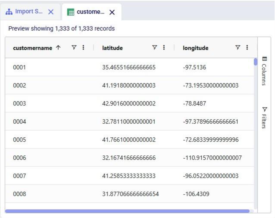
We have a look at the customers table which was created from the historical shipment data in the previous 2 quick start guides, see the screenshot below. Sorting on the customername column, we see that they are ordered in alphabetical order. This is because the customer name column is of type text as it starts with the string “CZ”. This leads to them not being ordered based on the number part that follows the “CZ” prefix.

If we want ordering customer names alphabetically to result in an order that is the same as sorting the number part of the customer name, we need to make sure each customer name has the same number of digits. We will use Update tasks to change the format of the number part of the customer names so that they are all 4 digits by adding leading 0’s to those that have less than 4 digits. While we are at it, we will also replace the “CZ” prefix with “Cust_” to make the data consistent with other data sources that contain customer names. We will break the updates to the customer name column up into 3 steps using 3 Update tasks initially. At the end, we will see how they can be combined into a single Update task. The 3 steps are:
Let us add the first Update task to our Import Shipments macro:
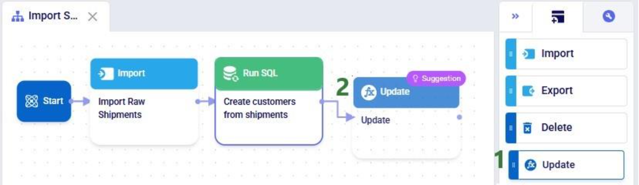
After dropping the Update task onto the macro canvas, its configuration tab will be opened automatically on the right-hand side:

If you have not already, click on the plus button to add your first update statement:
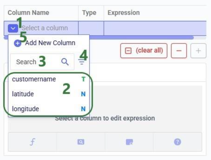
Next, we will write the expression for which we can use the Expression Builder area just below the update statements table. What we type there will also be added to the Expression column of the selected Update Statement. These expressions can use any PostgreSQL function, also those which may not be pre-populated in the helper lists. Please see the PostgreSQL documentation for all available functions.
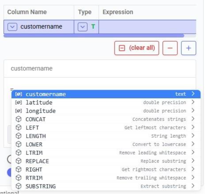
When clicking in the Expression Builder, an equal sign is already there, and a list of items comes up. At the top are the columns that are present in the target table and below those is a list of string functions which we can select to use. Here, the functions shown are string functions, since we are working on a text type column, when working on column with a different data type, other functions, those relevant to the data type, will be shown. We will select the last option shown in the screenshot, the substring function, since we want to first remove the “CZ” from the start of the customer names:
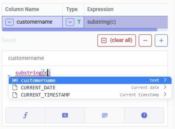
The substring function needs at least 2 arguments, which will be specified in the parentheses. The first argument needs to be the customername column in our case, since that is the column containing the string values we want manipulate. After typing a “c”, the customername column and 2 functions starting with “c” are suggested in the pop-up list. We choose the customername column. The second argument specifies the start location from where we want to start the substring. Since we want to remove the “CZ”, we specify 3 as the start location, leaving characters number 1 and 2 off. The third argument is optional; it indicates the end location of the substring. We do not specify it, meaning we want to keep all characters starting from character number 3:

We can run this task now without specifying a Condition (see section further below) in which case the expression will be applied to all records in the customers table. After running the task, we open the customers table to see the result:

We see that our intended change was made. The “CZ” is removed from the customer names. Sorted alphabetically, they still are not in increasing order of the number part of their name. Next, we use the lpad (left pad) function to add leading zeroes so all customer names consist of 4 digits. This function has 3 arguments: the string to apply the left padding to (the customername column), the number of characters the final string needs to have (4), and the padding character (‘0’).

After running this task, the customername column values are as follows:
Now with the leading zeroes and all customer names being 4 characters long, sorting alphabetically results in the same order as sorting by the number part of the customer name.
Finally, we want to add the prefix “Cust_”. We use the concat (concatenation) function for this. At first, we type Cust_ with double quotes around it, but the squiggly red line below the expression in the expression builder indicates this is not the right syntax. Hovering over the expression in the expression builder explains the problem:

The correct syntax for using strings in these functions is to use single quotes:
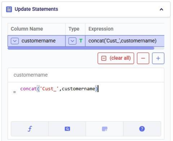
Instead of concat we can also use “= ‘Cust_’ || customername” as the expression. The double pipe symbol is used in PostgreSQL as the concatenation operator.
Running this third update task results in the following customer names in the customers table:
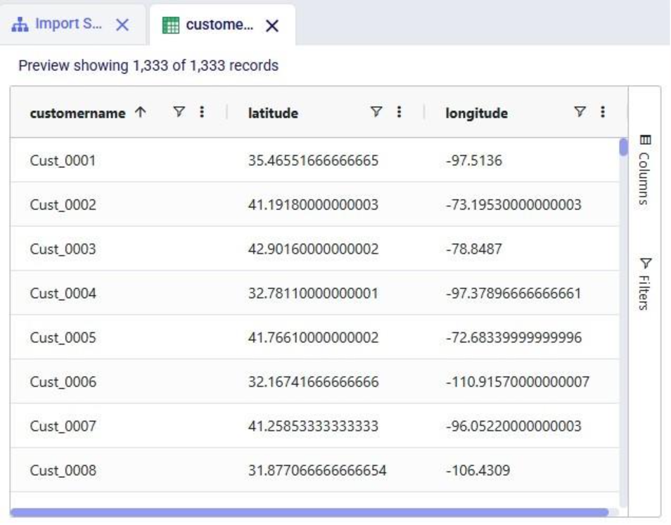
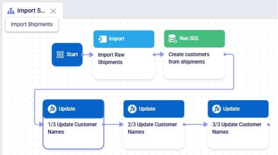
Our goal of how we wanted to update the customername column has been achieved. Our macro now looks as follows with the 3 Update tasks added:
The 3 tasks described above can be combined into 1 Update task by nesting the expressions as follows:

Running this task instead of the 3 above will result in the same changes to the customername column in the customers table.
Please note that in the above we only specified one update statement in each Update task. You can add more than one update statement per update task, in which case:
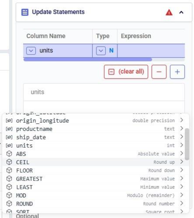
As mentioned above, the list of suggested functions is different depending on the data type of the column being updated. This screenshot shows part of the suggested functions for a number column:
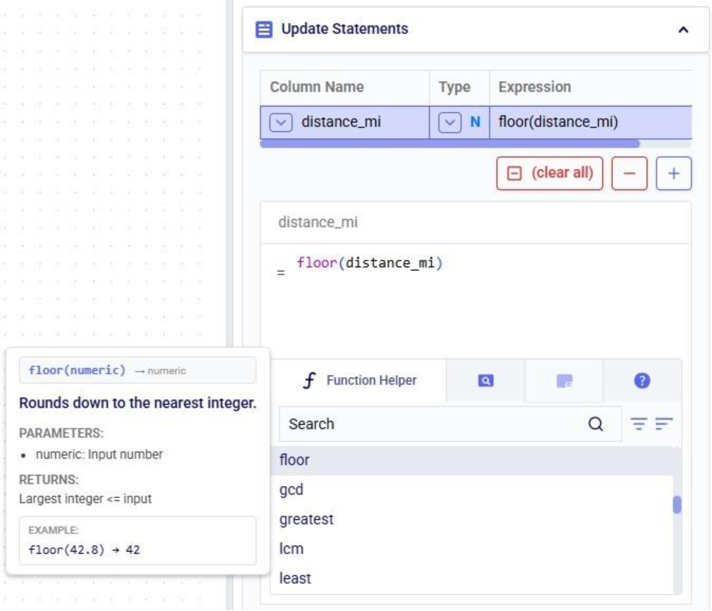
At the bottom of Expression Builder are multiple helper tabs to facilitate quickly building your desired expressions. The first one is the Function Helper which lists the available functions. The functions are listed by category: string, numeric, date, aggregate, and conditional. At the top of the list user has search, filter and sort options available to quickly find a function of interest. Hovering over a function in the list will bring up details of the function, from top to bottom: a summary of the format and input and output data types of the function, a description of what the function does, its input parameter(s), what it returns, and an example:
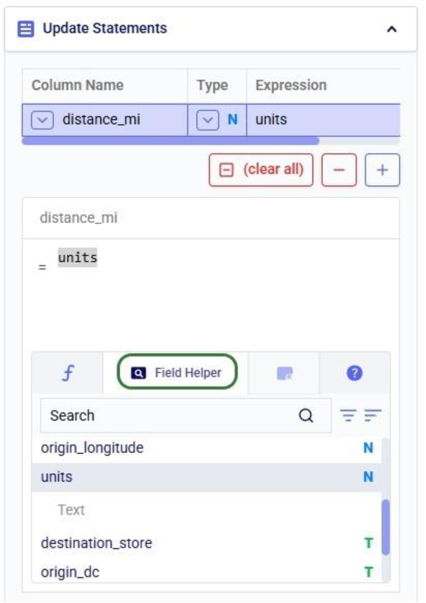
The next helper tab contains the Field Helper. This lists all the columns of the target table, sorted by their data type. Again, to quickly find the desired field, users can search, filter, and sort the list using the options at the top of the list:
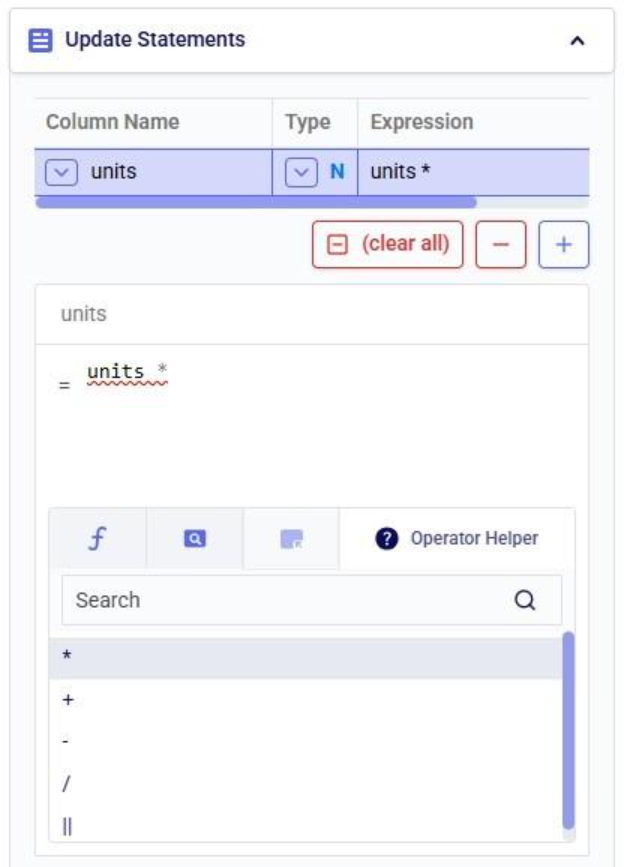
The fourth tab is the Operator Helper, which lists several helpful numerical and string operators. This list can be searched too using the Search box at the top of the list:
There is another optional configuration section for Update tasks, the Condition section. In here, users can specify an expression to filter the target table on before applying the update(s) specified in the Update Statements section. This way, the updates are only applied to the subset of records that match the condition.
In this example, we will look at some records of the rawshipments table in the project sandbox of the same project (“Import Historical Shipments). We have opened this table in a grid and filtered for origin_dc Salt Lake City DC and destination_store CZ103.

What we want to do is update the “units” column and increase the values by 50% for the Table product. The Update Statements section shows that we set the units field to its current value multiplied by 1.5, which will achieve the 50% increase:

However, if we run the Update task as is, all values in the units field will be increased by 50%, for both the Table and the Chair product. To make sure we only apply this increase to the Table product, we configure the Condition section as follows:
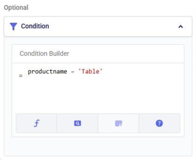
The condition builder has the same function, field, and operator helper tabs at the bottom as the expression builder in the update statements section to enable users to quickly build their conditions. Building conditions works in the same way as building expressions.
Running the task and checking the updated rawshipments table for the same subset of records as we saw above, we can check that it worked as intended. The values in the units column for the Table records are indeed 1.5 times their original value, while the Chair units are unchanged.
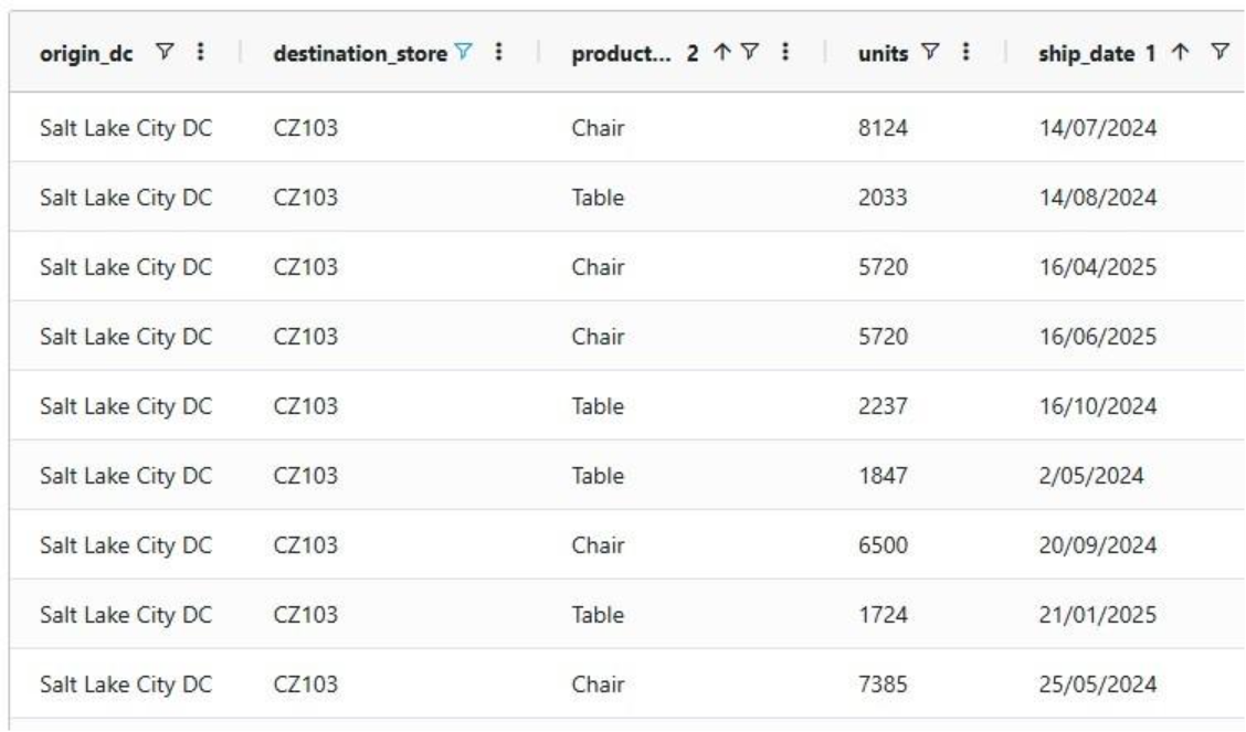
It is important to note that opening tables in DataStar currently shows a preview of 10,000 records. When filtering a table by clicking on the filter icons to the right of a column name, only the resulting subset of records from those first 10,000 records will be included. While an Update task will be applied to all records in a table, due to this limit on the number of records in the preview you may not always be able to see (all) results of your Update task in the grid. In addition, an Update task can also change the order of the records in the table. This can lead to a filter showing a different set of records after running an update task as compared to the filtered subset that was shown prior to running it. Users can use the SQL Editor application on the Optilogic platform to see the full set of records for any tables.
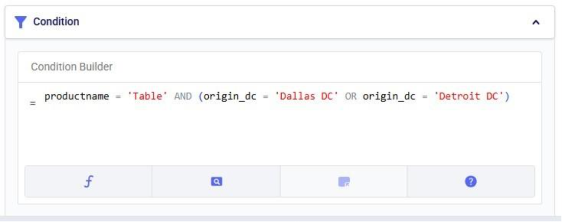
Finally, if you want to apply multiple conditions you can use logical AND and OR statements to combine them in the Expression Builder. You would for example specify the condition as follows if you want to increase the units for the Table product by 50% only for the records where the origin_dc value is either “Dallas DC” or “Detroit DC”:
In this quick start guide we will show how users can seamlessly go from using the Resource Library, Cosmic Frog and DataStar applications on the Optilogic platform to creating visualizations in Power BI. The example covers cost to serve analysis using a global sourcing model. We will run 2 scenarios in this Cosmic Frog model with the goal to visualize the total cost difference between the scenarios by customer on a map. We do this by coloring the customers based on the cost difference.
The steps we will walk through are:
We will first copy the model named “Global Sourcing – Cost to Serve” from the Resource Library to our Optilogic account (learn more about the Resource Library in this help center article):
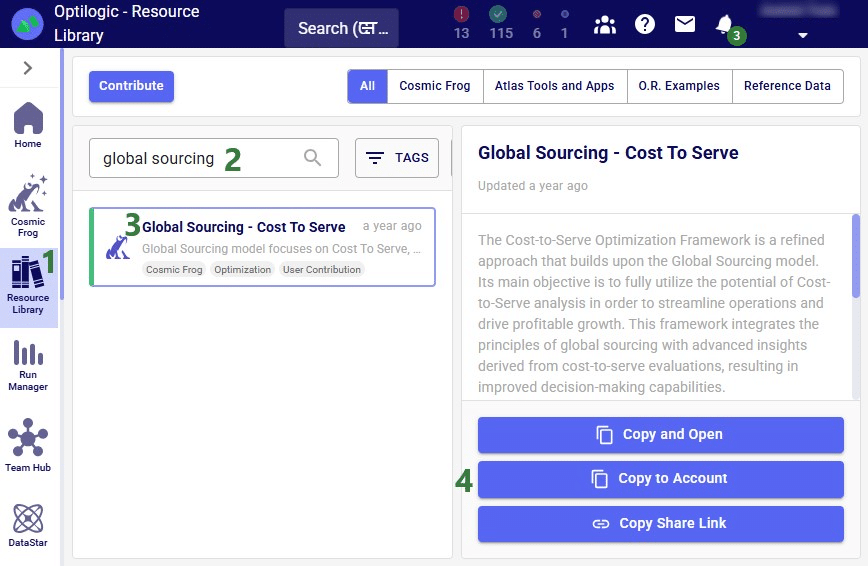
On the Optilogic platform, go to the Resource Library application by clicking on its icon in the list of applications on the left-hand side; note that you may need to scroll down. Should you not see the Resource Library icon here, then click on the icon with 3 horizontal dots which will then show all applications that were previously hidden too.
Now that the model is in the user’s account, it can be opened in the Cosmic Frog application:


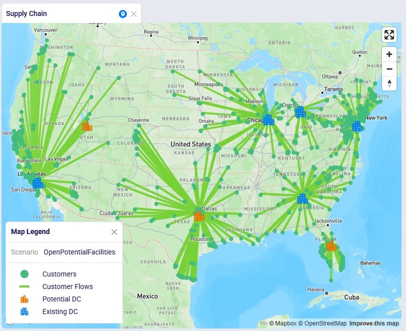
We will only have a brief look at some high-level outputs in Cosmic Frog in this quick start guide, but feel free to explore additional outputs. You can learn more about Cosmic Frog through these help center articles. Let us have a quick look at the Optimization Network Summary output table and the map:

Our next step is to import the needed input table and output table of the Global Sourcing – Cost to Serve model into DataStar. Open the DataStar application on the Optilogic platform by clicking on its icon in the applications list on the left-hand side. In DataStar, we first create a new project named “Cost to Serve Analysis” and set up a data connection to the Global Sourcing – Cost to Serve model, which we will call “Global Sourcing C2S CF Model”. See the Creating Projects & Data Connections section in the Getting Started with DataStar help center article on how to create projects and data connections. Then, we want to create a macro which will calculate the increase/decrease in total cost by customer between the 2 scenarios. We build this macro as follows:

The configuration of the first import task, C2S Path Summary, is shown in this screenshot:

The configuration of the other import task, Customers, uses the same Source Data Connection, but instead of the optimizationcosttoservepathsummary table, we choose the customers table as the table to import. Again, the Project Sandbox is the Destination Data Connection, and the new table is simply called customers.
Instead of writing SQL queries ourselves to pivot the data in the cost to serve path summary table to create a new table where for each customer there is a row which has the customer name and the total cost for each scenario, we can use Leapfrog to do it for us. See the Leapfrog section in the Getting Started with DataStar help center article and this quick start guide on using natural language to create DataStar tasks to learn more about using Leapfrog in DataStar effectively. For the Pivot Total Cost by Scenario by Customer task, the 2 Leapfrog prompts that were used to create the task are shown in the following screenshot:

The SQL Script reads:
DROP TABLE IF EXISTS total_cost_by_customer_combined;
CREATE TABLE total_cost_by_customer_combined AS
SELECT
  pathdestination AS customer,
  SUM(CASE WHEN scenarioname = 'Baseline' THEN pathcost ELSE 0 END)
    AS total_cost_baseline,
  SUM(CASE WHEN scenarioname = 'OpenPotentialFacilities' THEN pathcost ELSE 0 END)
    AS total_cost_openpotentialfacilities
FROM c2s_path_summary
WHERE scenarioname IN ('Baseline', 'OpenPotentialFacilities')
GROUP BY pathdestination
ORDER BY pathdestination;
To create the Calculate Cost Savings by Customer task, we gave Leapfrog the following prompt: “Use the total cost by customer table and add a column to calculate cost savings as the baseline cost minus the openpotentalfacilities cost”. The resulting SQL Script reads as follows:
ALTER TABLE total_cost_by_customer_combined
ADD COLUMN cost_savings DOUBLE PRECISION;
UPDATE total_cost_by_customer_combined
SET
cost_savings = total_cost_baseline - total_cost_openpotentialfacilities;
This task is also added to the macro; its name is "Calculate Cost Savings by Customer".
Lastly, we give Leapfrog the following prompt to join the table with cost savings (total_cost_by_customer_combined) and the customers table to add the coordinates from the customers table to the cost savings table: “Join the customers and total_cost_by_customer_combined tables on customer and add the latitude and longitude columns from the customers table to the total_cost_by_customer_combined table. Use an inner join and do not create a new table, add the columns to the existing total_cost_by_customer_combined table”. This is the resulting SQL Script, which was added to the macro as the "Add Coordinates to Cost Savings" task:
ALTER TABLE total_cost_by_customer_combined ADD COLUMN latitude VARCHAR;
ALTER TABLE total_cost_by_customer_combined ADD COLUMN longitude VARCHAR;
UPDATE total_cost_by_customer_combined SET latitude = c.latitude
FROM customers AS c
WHERE total_cost_by_customer_combined.customer = c.customername;
UPDATE total_cost_by_customer_combined SET longitude = c.longitude
FROM customers AS c
WHERE total_cost_by_customer_combined.customer = c.customername;
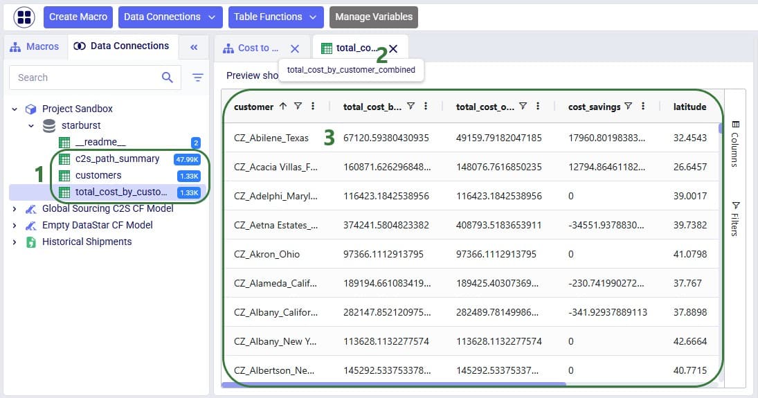
We can now run the macro, and once it is completed, we take a look at the tables present in the Project Sandbox:
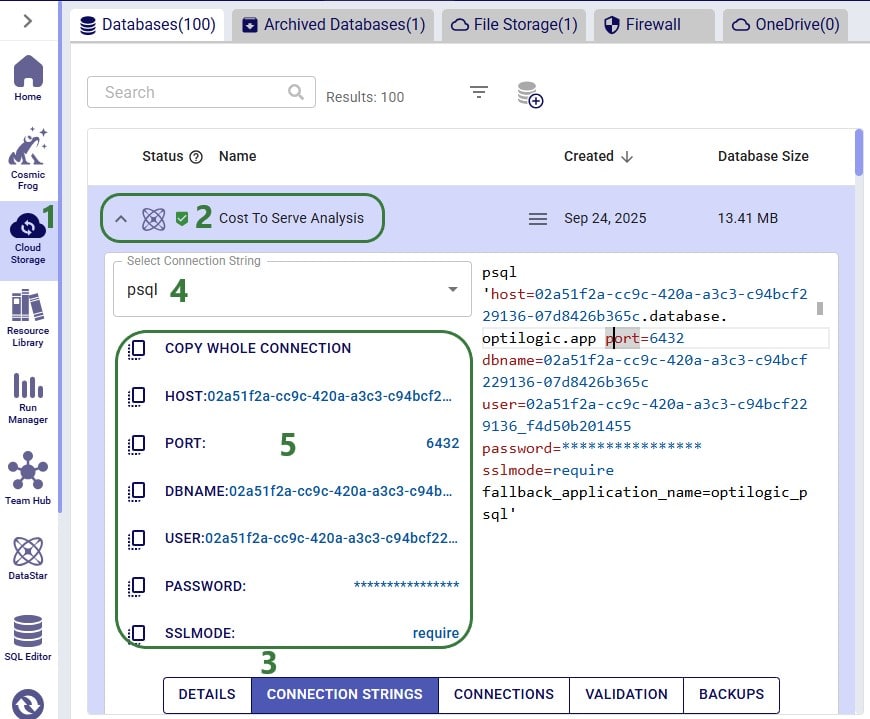
We will use Microsoft Power BI to visualize the change in total cost between the 2 scenarios by customer on a map. To do so, we first need to set up a connection to the DataStar project sandbox from within Power BI. Please follow the steps in the “Connecting to Optilogic with Microsoft Power BI” help center article to create this connection. Here we will just show the step to get the connection information for the DataStar Project Sandbox, which underneath is a PostgreSQL database (next screenshot) and selecting the table(s) to use in Power BI on the Navigator screen (screenshot after this one):
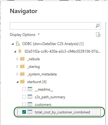
After selecting the connection within Power BI and providing the credentials again, on the Navigator screen, choose to use just the total_cost_by_customer_combined table as this one has all the information needed for the visualization:
We will set up the visualization on a map using the total_cost_by_customer_combined table that we have just selected for use in Power BI using the following steps:
With the above configuration, the map will look as follows:
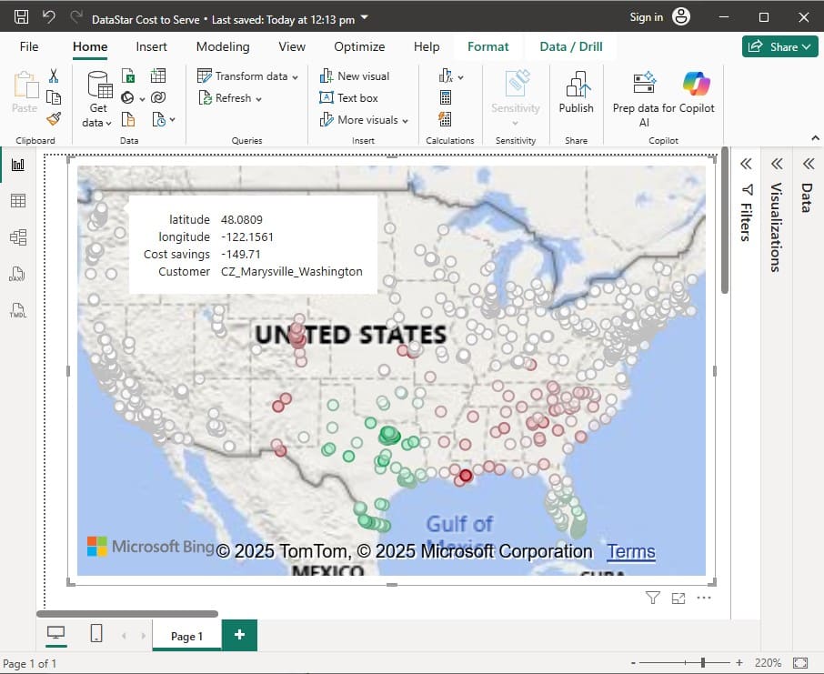
Green customers are those where the total cost went down in the OpenPotentialFacilities scenario, i.e. there are savings for this customer. The darker the green, the higher the savings. White customers did not see a lot of difference in their total costs between the 2 scenarios. The one that is hovered over, in Marysville in Washington state, has a small increase of $149.71 in total costs in the OpenPotentialFacilities scenario as compared to the Baseline scenario. Red customers are those where the total cost went up in the OpenPotentialFacilities scenario (i.e. the cost savings are a negative number); the darker the red, the higher the increase in total costs. As expected, the customers with the highest cost savings (darkest green) are those located in Texas and Florida, as they are now being served from DCs closer to them.
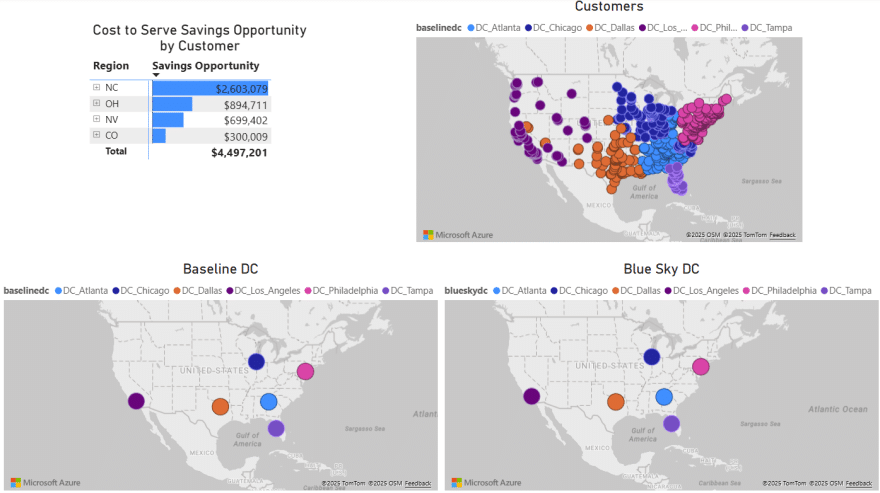
To give users an idea of what type of visualization and interactivity is possible within Power BI, we will briefly cover the 2 following screenshots. These are of a different Cosmic Frog model for which a cost to serve analysis is performed too. Two scenarios were run in this model: Baseline DC and Blue Sky DC. In the Baseline scenario, customers are assigned to their current DCs and in the Blue Sky scenario, they can be re-assigned to other DCs. The chart on the top left shows the cost savings by region (= US state) that are identified in the Blue Sky DC scenario. The other visualizations on the dashboard are all on maps: the top right map shows the customers which are colored based on which DC serves them in the Baseline scenario, the bottom 2 maps shows the DCs used in the Baseline (left) and the DCs used in the Blue Sky scenario.
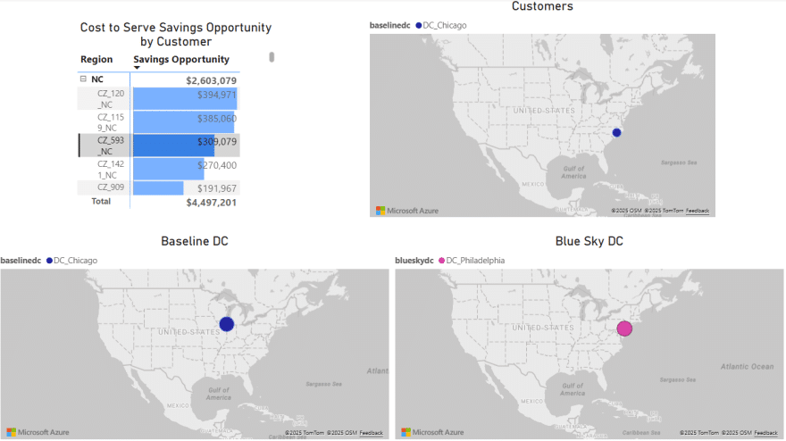
To drill into the differences between the 2 scenarios, users can expand the regions in the top left chart and select 1 or multiple individual customers. This is an interactive chart, and the 3 maps are then automatically filtered for the selected location(s). In the below screenshot, the user has expanded the NC region and then selected customer CZ_593_NC in the top left chart. In this chart, we see that the cost savings for this customer in the Blue Sky DC scenario as compared to the Baseline scenario amount to $309k. From the Customers map (top right) and Baseline DC map (bottom left) we see that this customer was served from the Chicago DC in the Baseline. We can tell from the Blue Sky DC map (bottom right) that this customer is re-assigned to be served from the Philadelphia DC in the Blue Sky DC scenario.
Optilogic has developed Python libraries to facilitate scripting for 2 of its flagship applications: Cosmic Frog, the most powerful supply chain design tool on the market, and DataStar, its just released AI-powered data product where users can create flexible, accessible and repeatable workflows with zero learning curve.
Instead of going into the applications themselves to build and run supply chain models and data workflows, these libraries enable users to programmatically access their functionality and underlying data. Example use cases for such scripts are:
In this documentation we cover the basics of getting yourself set up so you can take advantage of these Python scripting libraries, both on a local computer and on the Optilogic platform leveraging the Lightning Editor application. More specific details for the cosmicfrog and datastar libraries, including examples and end-to-end scripts, are detailed in the following Help Center articles and library specifications:
Working locally with Python scripts has the advantage that you can make use of code completion features which may include text auto-completion, showing what arguments functions need, catching incorrect syntax/names, etc. An example set up to achieve this is for example one where Python, Visual Studio Code, and an IntelliSense extension package for Python for Visual Studio Code are installed locally:
Once you are set up locally and are starting to work with Python scripts in Visual Studio Code, you will need to install the Python libraries you want to use to have access to their functionality. You do this by typing following in a terminal in Visual Studio Code (if no terminal is open yet: click on the View menu at the top and select Terminal, or the keyboard shortcut Ctrl + ` can be used):
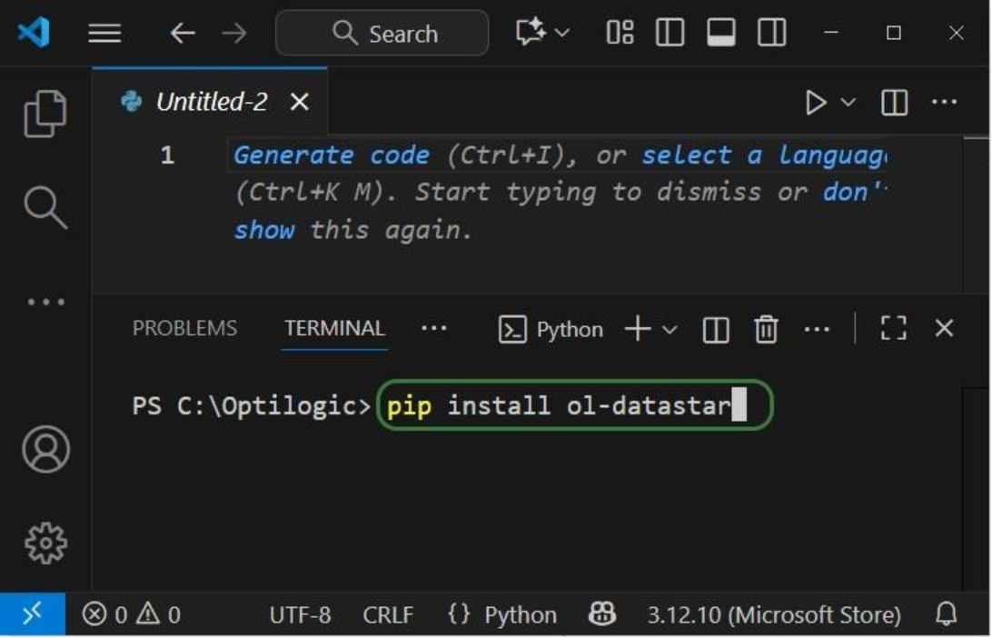
When installing these libraries, multiple external libraries (dependencies) are installed too. These are required to run the packages successfully and/or make working with them easier. These include the optilogic, pandas, and SQLAlchemy packages (among others) for both libraries. You can find out which packages are installed with the cosmicfrog / ol-datastar libraries by typing “pip show cosmicfrog” or “pip show ol-datastar" in a terminal.
To use other Python libraries in addition, you will usually need to install them using “pip install” too before you can leverage them.
If you want to access certain items on the Optilogic platform (like Cosmic Frog models, DataStar project sandboxes) while working locally, you will need to whitelist your IP address on the platform, so the connections are not blocked by a firewall. You can do this yourself on the Optilogic platform:

Please note that for working with DataStar, the whitelisting of your IP address is only necessary if you want to access the Project Sandbox of projects directly through scripts. You do not need to whitelist your IP address to leverage other functions while scripting, like creating projects, adding macros and their tasks, and running macros.
App Keys are used to authenticate the user from the local environment on the Optilogic platform. To create an App Key, see this Help Center Article on Generating App and API Keys. Copy the generated App Key and paste it into an empty Notepad window. Save this file as app.key and place it in the same folder as your local Python script.
It is important to emphasize that App Keys and app.key files should not be shared with others, e.g. remove them from folders / zip-files before sharing. Individual users need to authenticate with their own App Key.
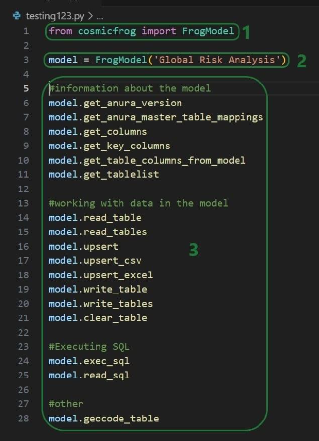
The next set of screenshots will show an example Python script named testing123.py on our local set-up. Here it uses the cosmicfrog library, using the ol-datastar library works similarly. The first screenshot shows a list of functions available from the cosmicfrog Python library:
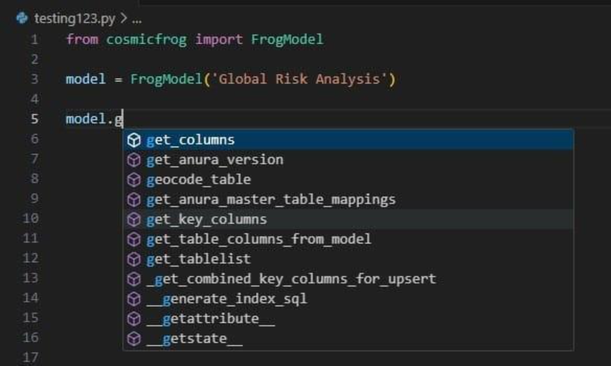
When you continue typing after you have typed “model.” the code completion feature will auto-generate a list of functions you may be getting at. In the next screenshot ones that start with or contain a “g” as I have only typed a “g” so far. This list will auto-update the more you type. You can select from the list with your cursor or arrow up/down keys and hitting the Tab key to select and auto-complete:
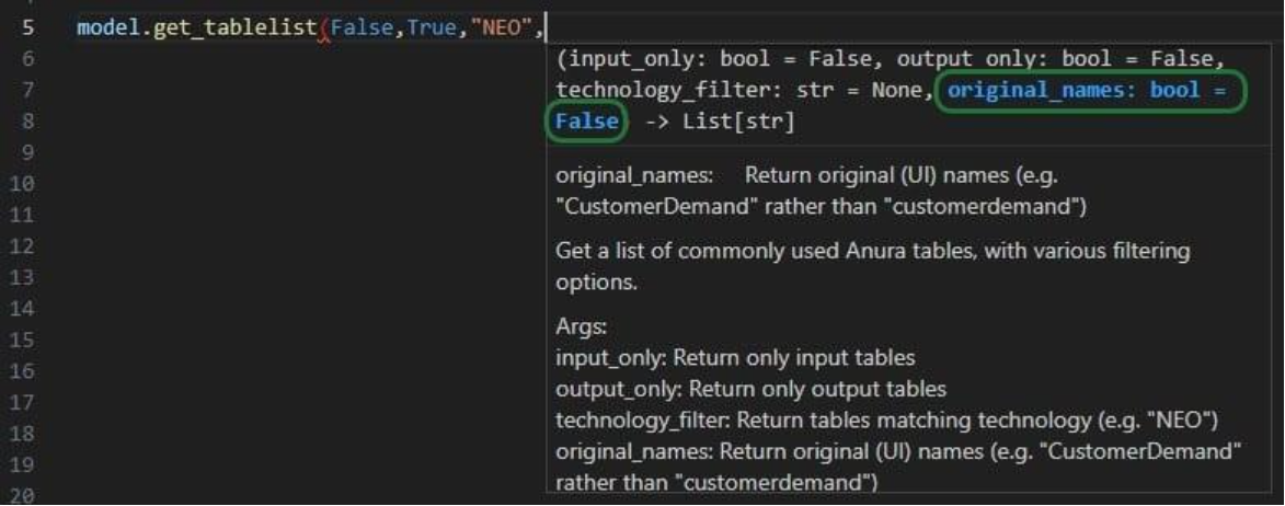
When you have completed typing the function name and next type a parenthesis ‘(‘ to start entering arguments, a pop-up will come up which contains information about the function and its arguments:
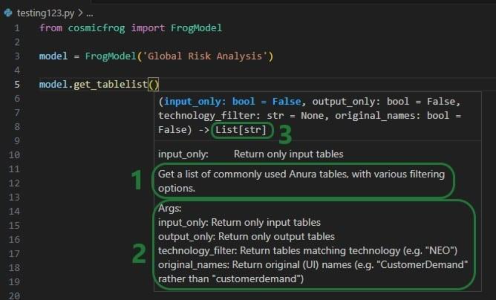
As you type the arguments for the function, the argument that you are on and the expected format (e.g. bool for a Boolean, str for string, etc.) will be in blue font and a description of this specific argument appears above the function description (e.g. above box 1 in the above screenshot). In the screenshot above we are on the first argument input_only which requires a Boolean as input and will be set to False by default if the argument is not specified. In the screenshot below we are on the fourth argument (original_names) which is now in blue font; its default is also False, and the argument description above the function description has changed now to reflect the fourth argument:
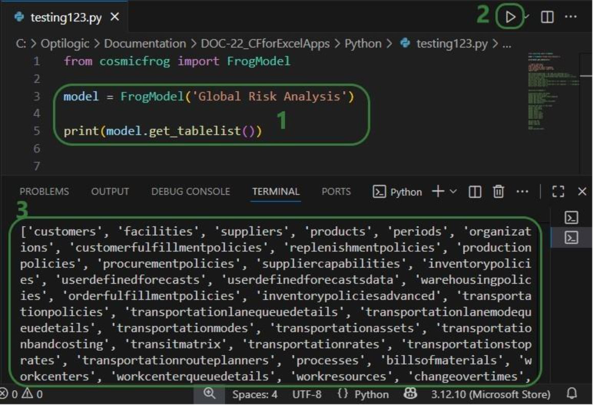
Once you are ready to run a script, you can click on the play button at the top right of the screen:
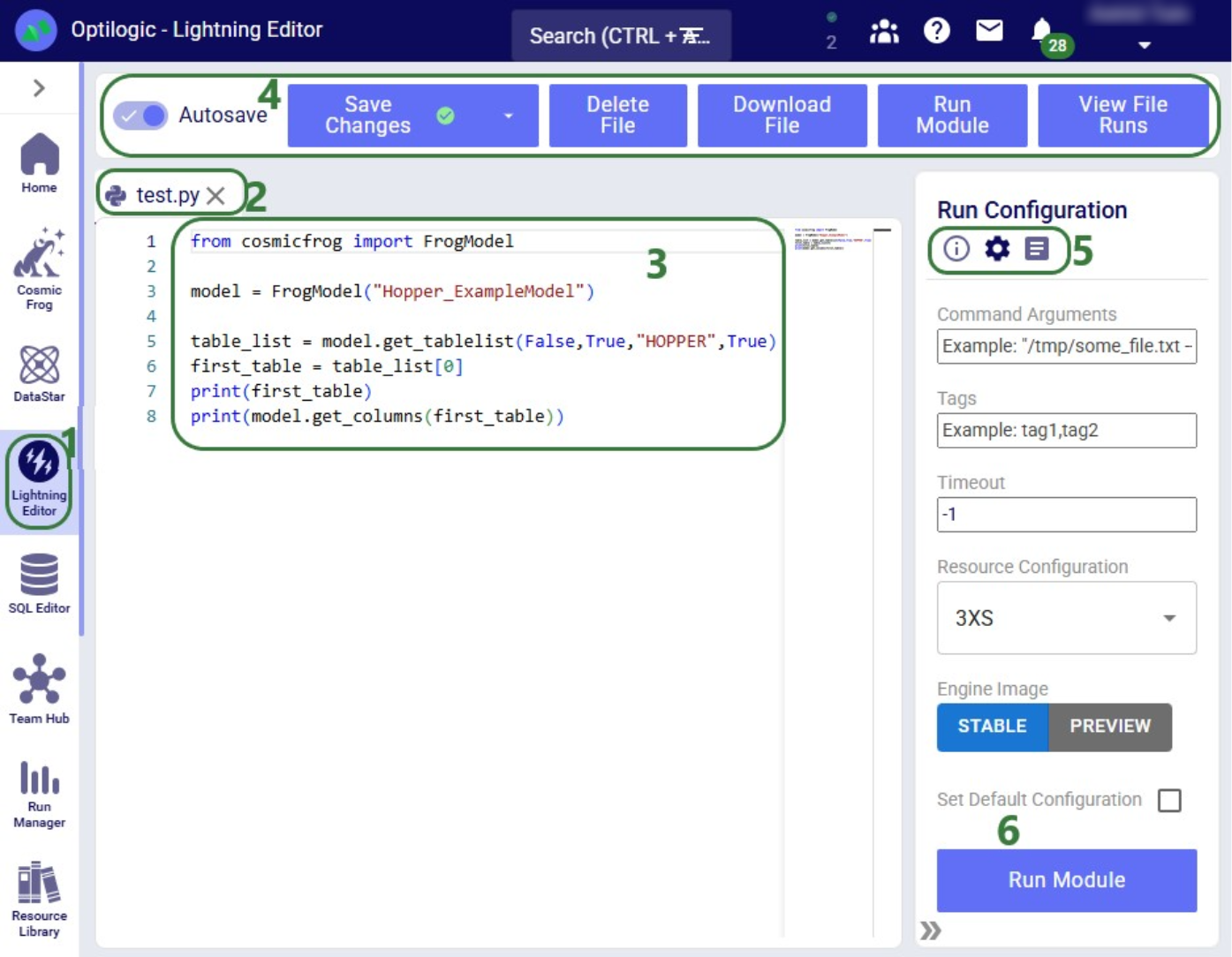
As mentioned above, you can also use the Lightning Editor application on the Optilogic platform to create and run Python scripts. Lightning Editor is an Integrated Development Environment (IDE) which has some code completion features, but these are not as extensive and complete as those in Visual Studio Code when used with an IntelliSense extension package.
When working on the Optilogic platform, you are already authenticated as a user, and you do not need to generate / provide an App Key or app.key file nor whitelist your IP address.
When using the datastar library in scripts, users need to place a requirements.txt file in the same folder on the Optilogic platform as the script. This file should only contain the text “ol-datastar” (without the quotes). No requirements.txt files is required when using the cosmicfrog library.
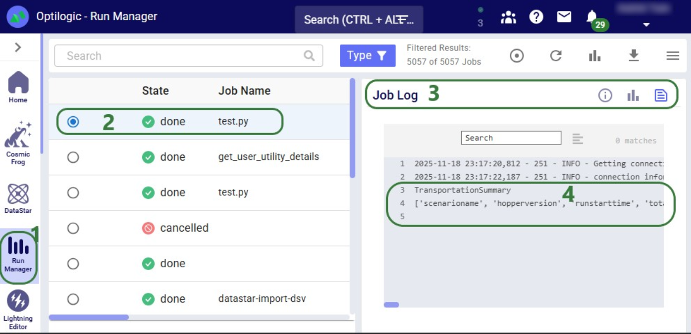
The following simple test.py Python script on Lightning Editor will print the first Hopper output table name and its column names:

DataStar users can take advantage of the datastar Python library, which gives users access to DataStar projects, macros, tasks, and connections through Python scripts. This way users can build, access, and run their DataStar workflows programmatically. The library can be used in a user’s own Python environment (local or on the Optilogic platform), and it can also be used in Run Python tasks in a DataStar macro.
In this documentation we will cover how to use the library through multiple examples. At the end, we will step through an end-to-end script that creates a new project, adds a macro to the project, and creates multiple tasks that are added to the macro. The script then runs the macro while giving regular updates on its progress.
Before diving into the details of this article, it is recommended to read this “Setup: Python Scripts for Cosmic Frog and DataStar” article first; it explains what users need to do in terms of setup before they can run Python scripts using the datastar library. To learn more about the DataStar application itself, please see these articles on Optilogic’s Help Center.
Succinct documentation in PDF format of all datastar library functionality can be downloaded here (please note that the long character string at the beginning of the filename is expected). This includes a list of all available properties and methods for the Project, Macro, Task, and Connection classes at the end of the document.
All Python code that is shown in the screenshots throughout this documentation is available in the Appendix, so that you can copy-paste from there if you want to run the exact same code in your own Python environment and/or use these as jumping off points for your own scripts.
If you have reviewed the “Setup: Python Scripts for Cosmic Frog and DataStar” article and are set up with your local or online Python environment, we are ready to dive in! First, we will see how we can interrogate existing projects and macros using Python and the datastar library. We want to find out which DataStar projects are already present in the user’s Optilogic account.
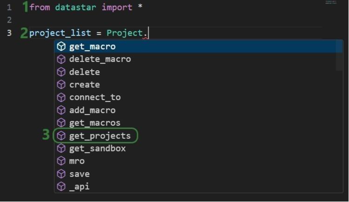

Once the parentheses are typed, hover text comes up with information about this function. It tells us that the outcome of this method will be a list of strings, and the description of the method reads “Retrieve all project names visible to the authenticated user”. Most methods will have similar hover text describing the method, the arguments it takes and their default values, and the output format.
Now that we have a variable that contains the list of DataStar projects in the user account, we want to view the value of this variable:
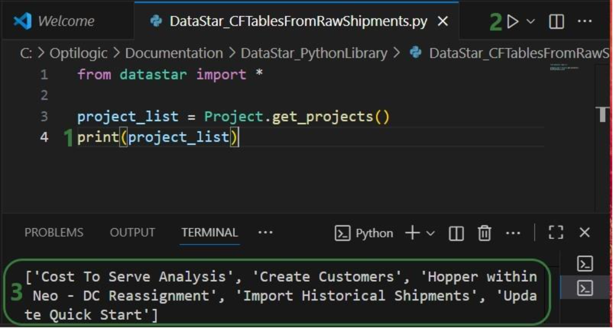
Next, we want to dig one level deeper and for the “Import Historical Shipments” project find out what macros it contains:

Finally, we will retrieve the tasks this “Import Shipments” macro contains in a similar fashion:
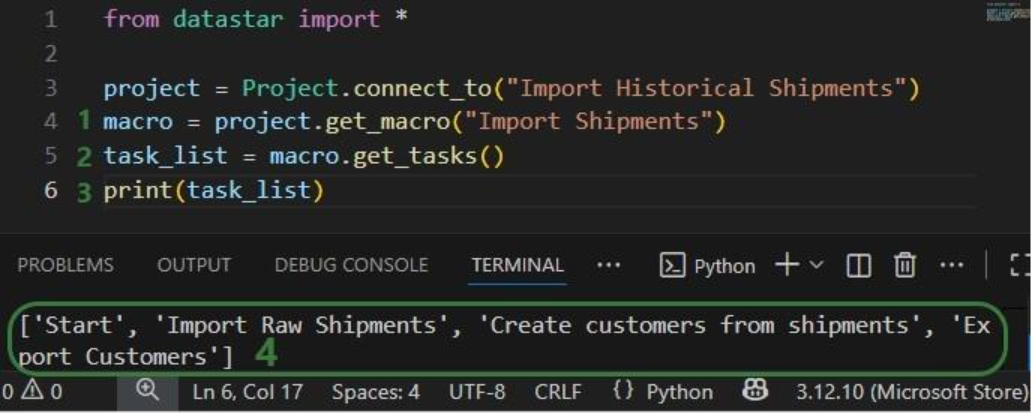
In addition, we can have a quick look in the DataStar application to see that the information we are getting from the small scripts above matches what we have in our account in terms of projects (first screenshot below), and the “Import Shipments” macro plus its tasks in the “Import Historical Shipments” project (second screenshot below):

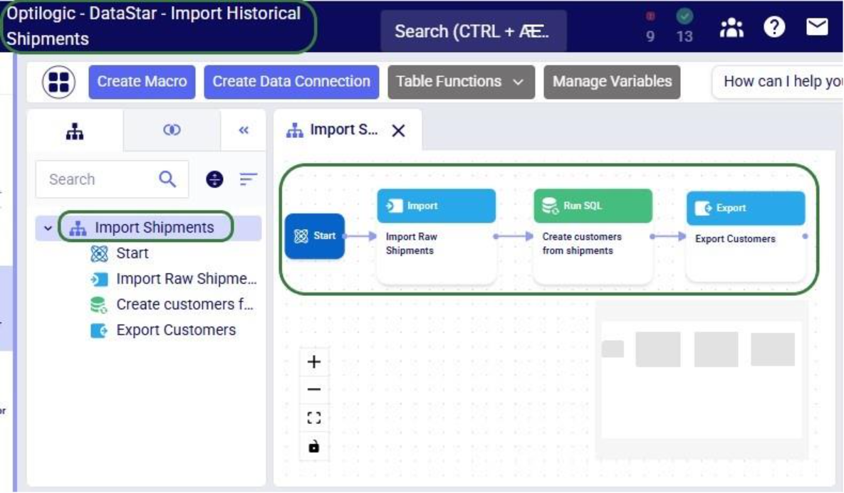
Besides getting information about projects and macros, other useful methods for projects and macros include:
Note that when creating new objects (projects, macros, tasks or connections) these are automatically saved. If existing objects are modified, their changes need to be committed by using the save method.
Macros can be copied, either within the same project or into a different project. Tasks can also be copied, either within the same macro, between macros in the same project, or between macros of different projects. If a task is copied within the same macro, its name will automatically be suffixed with (Copy).
As an example, we will consider a macro called “Cost Data” in a project named “Data Cleansing and Aggregation NA Model”, which is configured as follows:

The North America team shows this macro to their EMEA counterparts who realize that they could use part of this for their purposes, as their transportation cost data has the same format as that of the NA team. Instead of manually creating a new macro with new tasks that duplicate the 3 transportation cost related ones, they decide to use a script where first the whole macro is copied to a new project, and then the 4 tasks which are not relevant for the EMEA team are deleted:

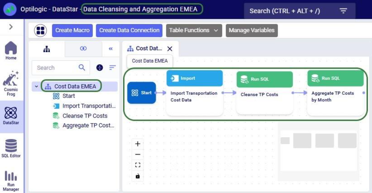
After running the script, we see in DataStar that there is indeed a new project named “Data Cleansing and Aggregation EMEA” which has a “Cost Data EMEA” macro that contains the 3 transportation cost related tasks that we wanted to keep:
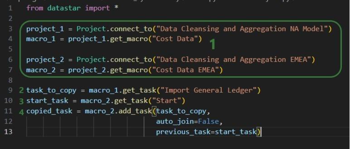
Note that another way we could have achieved this would have been to copy the 3 tasks from the macro in the NA project to the new macro in the EMEA project. The next example shows this for one task. Say that after the Cost Data EMEA macro was created, the team finds they also have a use for the “Import General Ledger” task that was deleted as it was not on the list of “tasks to keep”. In an extension of the previous script or a new one, we can leverage the add_task method of the Macro class to copy the “Import General Ledger” task from the NA project to the EMEA one:
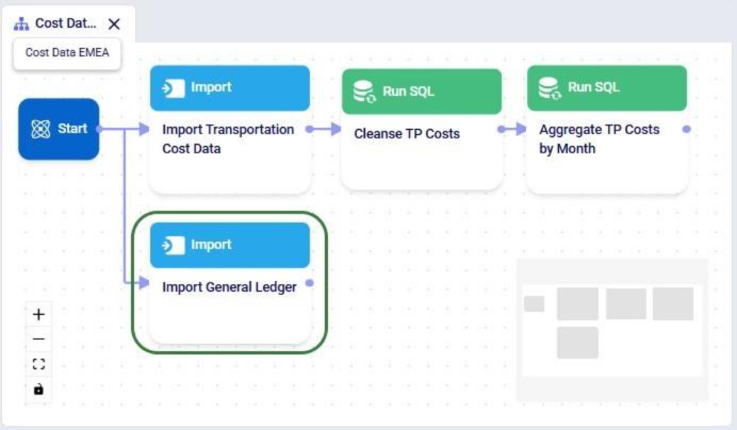
After running the script, we see that the “Import General Ledger” task is now part of the “Cost Data EMEA” macro and is connected to the Start task:
Several additional helpful features on chaining tasks together in a macro are:
DataStar connections allow users to connect to different types of data sources, including CSV-files, Excel files, Cosmic Frog models, and Postgres databases. These data sources need to be present on the Optilogic platform (i.e. visible in the Explorer application). They can then be used as sources / destinations / targets for tasks within DataStar.
We can use scripts to create data connections:
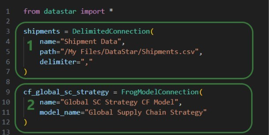
After running this script, we see the connections have been created. In the following screenshot, the Explorer is on the left, and it shows the Cosmic Frog model “Global Supply Chain Strategy.frog” and the Shipments.csv file. The connections using these are listed in the Data Connections tab of DataStar. Since we did not specify any description, an auto-generated description “Created by the Optilogic Datastar library” was added to each of these 2 connections:
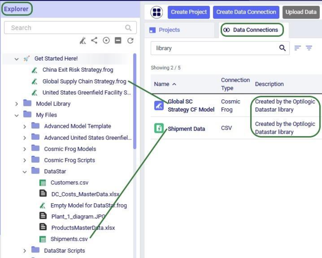
In addition to the connections shown above, data connections to Excel files (.xls and .xlsx) and PostgreSQL databases which are stored on the Optilogic platform can be created too. Use the ExcelConnection and OptiConnection classes to set up such these types of connections up.
Each DataStar project has its own internal data connection, the project sandbox. This is where users perform most of the data transformations after importing data into the sandbox. Using scripts, we can access and modify data in this sandbox directly instead of using tasks in macros to do so. Note that if you have a repeatable data workflow in DataStar which is used periodically to refresh a Cosmic Frog model where you update your data sources and re-run your macros, you need to be mindful of making one-off changes to the project sandbox through a script. When you change data in the sandbox through a script, macros and tasks are not updated to reflect these modifications. When running the data workflow the next time, the results may be different if that change the script made is not made again. If you want to include such changes in your macro, you can add a Run Python task to your macro within DataStar.
Our “Import Historical Shipments” project has a table named customers in its project sandbox:

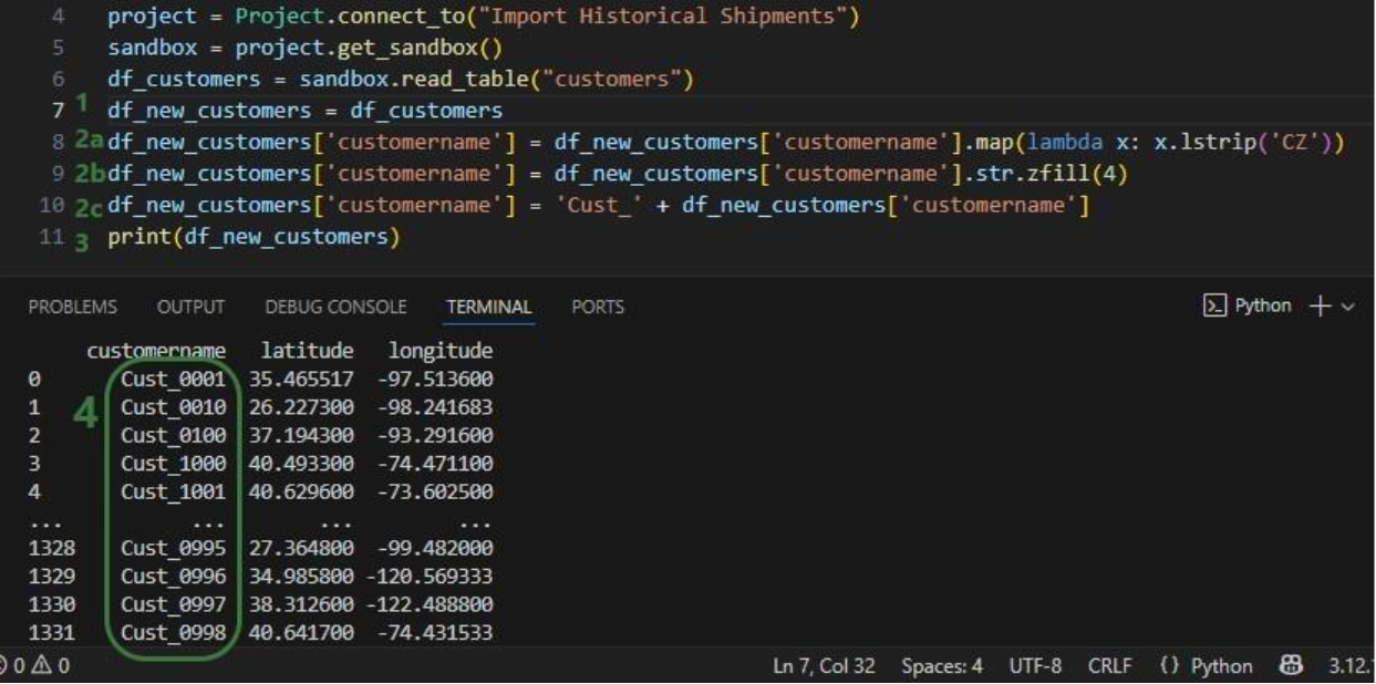
To make the customers sort in numerical order of their customer number, our goal in the next script is to update the number part of the customer names with left padded 0’s so all numbers consist of 4 digits. And while we are at it, we are also going to replace the “CZ” prefix with a “Cust_” prefix.
First, we will show how to access data in the project sandbox:
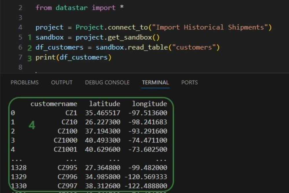
Next, we will use functionality of the pandas Python library (installed as a dependency when installing the datastar library) to transform the customer names to our desired Cust_xxxx format:
As a last step, we can now write the updated customer names back into the customers table in the sandbox. Or, if we want to preserve the data in the sandbox, we can also write to a new table as is done in the next screenshot:
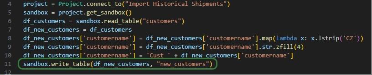
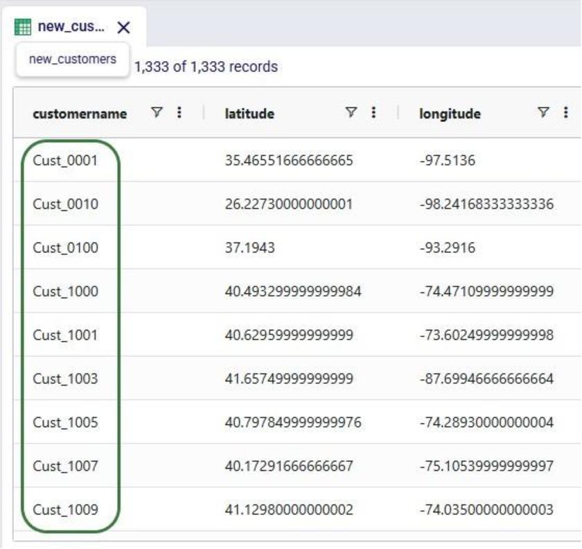
We use the write_table method to write the dataframe with the updated customer names into a new table called “new_customers” in the project sandbox. After running the script, opening this new table in DataStar shows us that the updates worked:
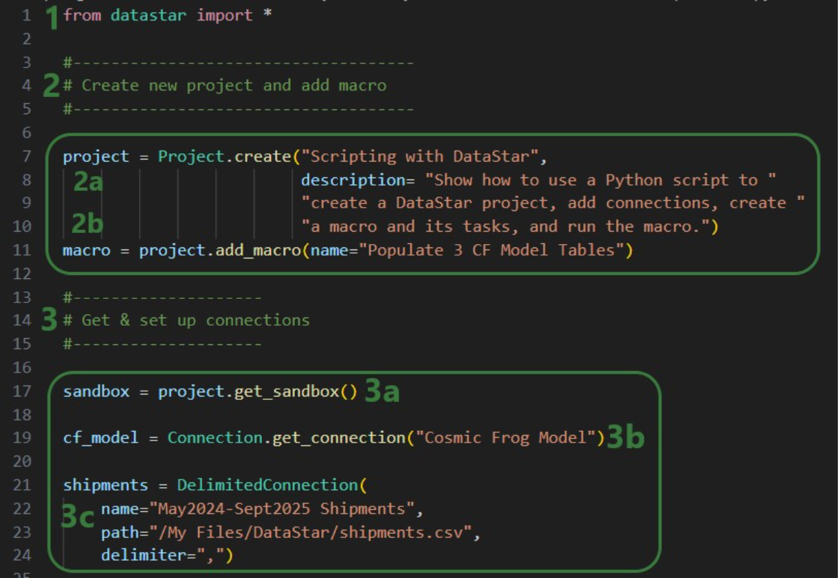
Finally, we will put everything we have covered above together in one script which will:
We will look at this script through the next set of screenshots. For those who would like to run this script themselves, and possibly use it as a starting point to modify into their own script:

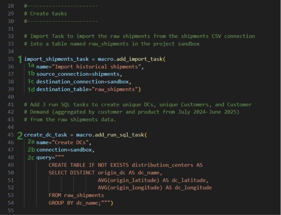
Next, we will create 7 tasks to add to the “Populate 3 CF Model Tables” macro, starting with an Import task:
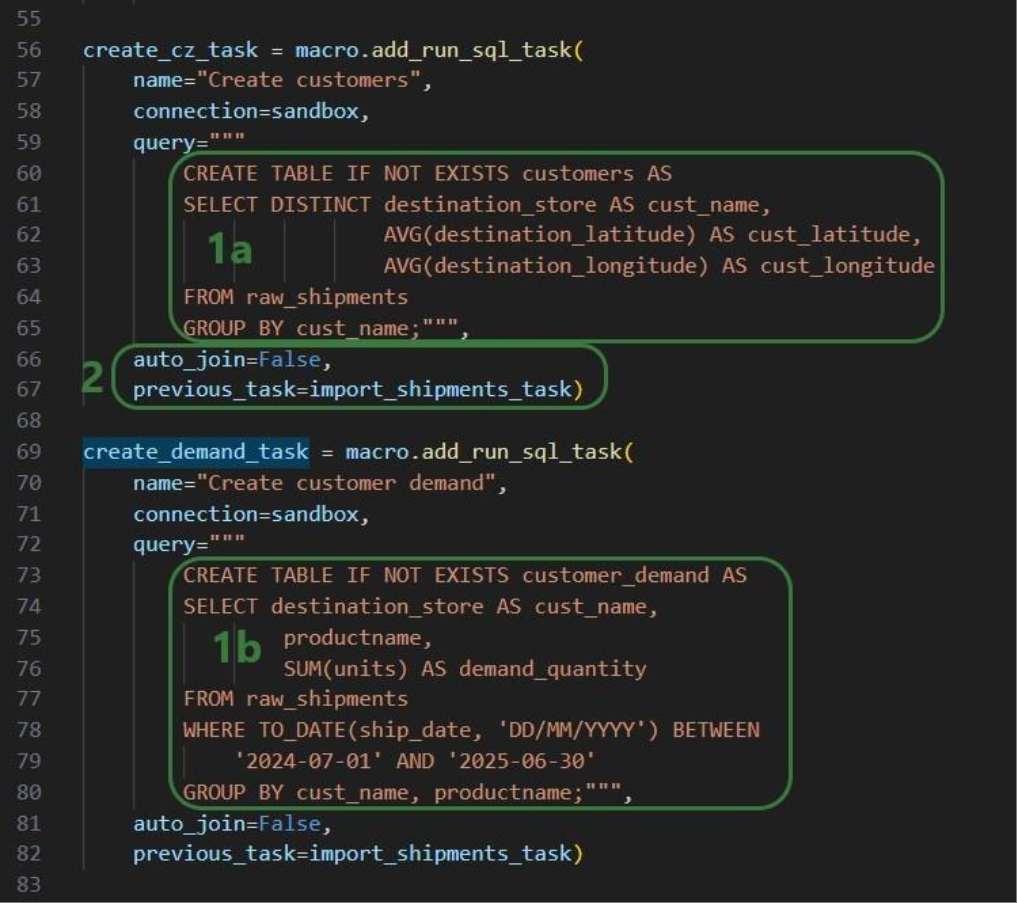
Similar to the “create_dc_task” Run SQL task, 2 more Run SQL tasks are created to create unique customers and aggregated customer demand from the raw_shipments table:
Now that we have generated the distribution_centers, customers, and customer_demand tables in the project sandbox using the 3 SQL Run tasks, we want to export these tables into their corresponding Cosmic Frog tables (facilities, customers, and customerdemand) in the empty Cosmic Frog model:
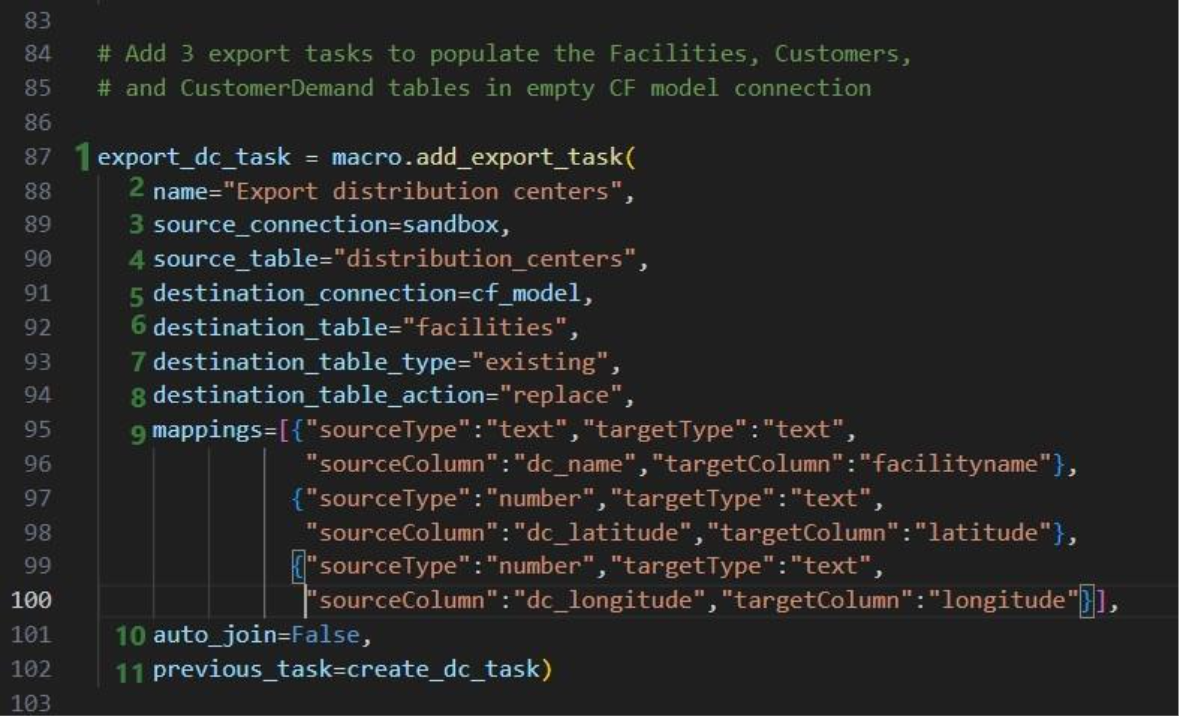
The following 2 Export tasks are created in a very similar way:
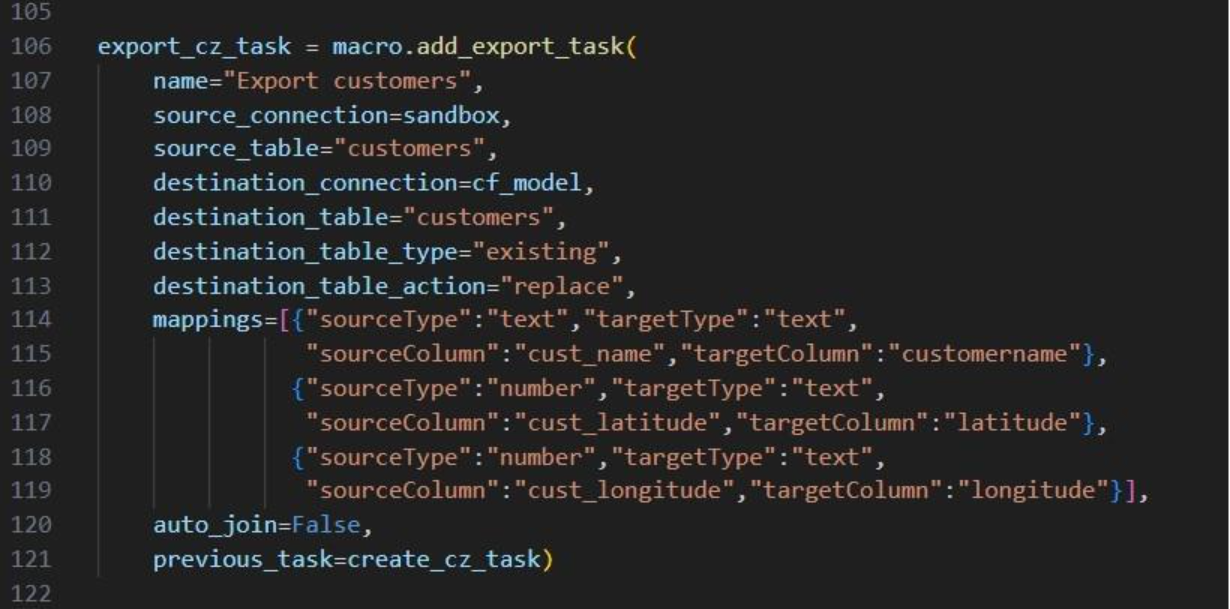
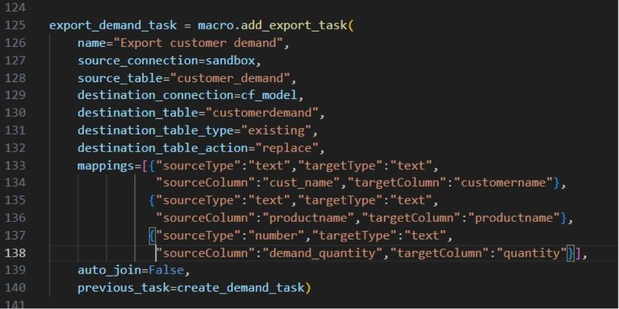
This completes the build of the macro and its tasks.
If we run it like this, the tasks will be chained in the correct way, but they will be displayed on top of each other on the Macro Canvas in DataStar. To arrange them nicely and prevent having to reposition them manually in the DataStar UI, we can use the “x” and “y” properties of tasks. Note that since we are now changing existing objects, we need to use the save method to commit the changes:
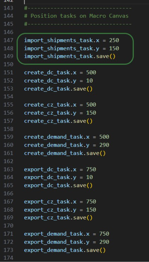
In the green outlined box, we see that the x-coordinate on the Macro Canvas for the import_shipments_task is set to 250 (line 147) and its y-coordinate to 150 (line 148). In line 149 we use the save method to persist these values.
Now we can kick off the macro run and monitor its progress:
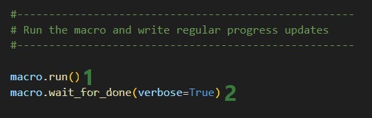
While the macro is running, messages written to the terminal by the wait_for_done method will look similar to following:
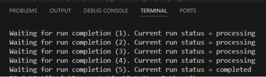
We see 4 messages where the status was “processing” and then a final fifth one stating the macro run has completed. Other statuses one might see are pending when the macro has not yet started and errored in case the macro could not finish successfully.
Opening the DataStar application, we can check the project and CSV connection were created on the DataStar startpage. They are indeed there, and we can open the “Scripting with DataStar” project to check the “Populate 3 CF Model Tables” macro and the results of its run:

The macro contains the 7 tasks we expect and checking their configurations shows they are set up the way we intended to.
Next, we have a look at the Data Connections tab to see the results of running the macro:
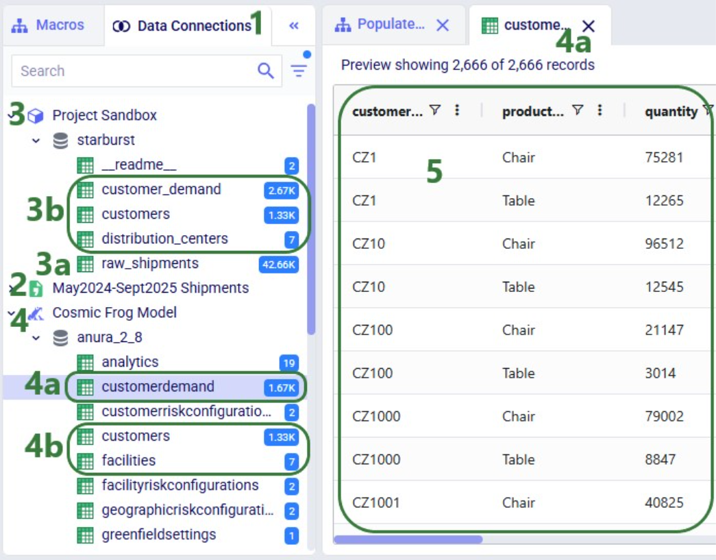
Here follows the code of each of the above examples. You can copy and paste this into your own scripts and modify them to your needs. Note that whenever names and paths are used, you may need to update these to match your own environment.
Get list of DataStar projects in user's Optilogic account and print list to terminal:
from datastar import *

project_list = Project.get_projects()
print(project_list)
Connect to the project named "Import Historical Shipments" and get the list of macros within this project. Print this list to the terminal:
from datastar import *

project = Project.connect_to("Import Historical Shipments")
macro_list = project.get_macros()
print(macro_list)
In the same "Import Historical Shipments" project, get the macro named "Import Shipments", and get the list of tasks within this macro. Print the list with task names to the terminal:
from datastar import *

project = Project.connect_to("Import Historical Shipments")
macro = project.get_macro("Import Shipments")
task_list = macro.get_tasks()
print(task_list)
Copy 3 of the 7 tasks in the "Cost Data" macro in the "Data Cleansing and Aggregation NA Model" project to a new macro "Cost Data EMEA" in a new project "Data Cleansing and Aggregation EMEA". Do this by first copying the whole macro and then removing the tasks that are not required in this new macro:
from datastar import *

# connect to project and get macro to be copied into new project
project = Project.connect_to("Data Cleansing and Aggregation NA Model")
macro = project.get_macro("Cost Data")

# create new project and clone macro into it
new_project = Project.create("Data Cleansing and Aggregation EMEA")
new_macro = macro.clone(new_project,name="Cost Data EMEA",
                        description="Cloned from NA project; \
                                    keep 3 transportation tasks")

# list the transportation cost related tasks to be kept and get a list
# of tasks present in the copied macro in the new project, so that we
# can determine which tasks to delete
tasks_to_keep = ["Start",
                 "Import Transportation Cost Data",
                 "Cleanse TP Costs",
                 "Aggregate TP Costs by Month"]
tasks_present = new_macro.get_tasks()

# go through tasks present in the new macro and
# delete if the task name is not in the "to keep" list
for task in tasks_present:
    if task not in tasks_to_keep:
        new_macro.delete_task(task)
Copy specific task "Import General Ledger" from the "Cost Data" macro in the "Data Cleansing and Aggregation NA Model" project to the "Cost Data EMEA" macro in the "Data Cleansing and Aggregation EMEA" project. Chain this copied task to the Start task:
from datastar import *

project_1 = Project.connect_to("Data Cleansing and Aggregation NA Model")
macro_1 = project_1.get_macro("Cost Data")

project_2 = Project.connect_to("Data Cleansing and Aggregation EMEA")
macro_2 = project_2.get_macro("Cost Data EMEA")

task_to_copy = macro_1.get_task("Import General Ledger")
start_task = macro_2.get_task("Start")
copied_task = macro_2.add_task(task_to_copy,
                               auto_join=False,
                               previous_task=start_task)
Creating a CSV file connection and a Cosmic Frog Model connection:
from datastar import *

shipments = DelimitedConnection(
    name="Shipment Data",
    path="/My Files/DataStar/Shipments.csv",
    delimiter=","
)

cf_global_sc_strategy = FrogModelConnection(
    name="Global SC Strategy CF Model",
    model_name="Global Supply Chain Strategy"
)
Connect directly to a project's sandbox, read data into a pandas dataframe, transform it, and write the new dataframe into a new table "new_customers":
from datastar import *

# connect to project and get its sandbox
project = Project.connect_to("Import Historical Shipments")
sandbox = project.get_sandbox()

# use pandas to raed the "customers" table into a dataframe
df_customers = sandbox.read_table("customers")

# copy the dataframe into a new dataframe
df_new_customers = df_customers

# use pandas to change the customername column values format
# from CZ1, CZ20, etc to Cust_0001, Cust_0020, etc
df_new_customers['customername'] = df_new_customers['customername'].map(lambda x: x.lstrip('CZ'))
df_new_customers['customername'] = df_new_customers['customername'].str.zfill(4)
df_new_customers['customername'] = 'Cust_' + df_new_customers['customername']

# write the updates customers table with the new customername
# values to a new table "new_customers"
sandbox.write_table(df_new_customers, "new_customers")
End-to-end script - create a new project and add a new macro to it; add 7 tasks to the macro to import shipments data; create unique customers, unique distribution centers, and demand aggregated by customer and product from it. Then export these 3 tables to a Cosmic Frog model:
from datastar import *

#------------------------------------
# Create new project and add macro
#------------------------------------

project = Project.create("Scripting with DataStar",
                         description= "Show how to use a Python script to "
                         "create a DataStar project, add connections, create "
                         "a macro and its tasks, and run the macro.")
macro = project.add_macro(name="Populate 3 CF Model Tables")

#--------------------
# Get & set up connections
#--------------------

sandbox = project.get_sandbox()

cf_model = Connection.get_connection("Cosmic Frog Model")

shipments = DelimitedConnection(
    name="May2024-Sept2025 Shipments",
    path="/My Files/DataStar/shipments.csv",
    delimiter=",")


#-----------------------
# Create tasks
#-----------------------

# Import Task to import the raw shipments from the shipments CSV connection
# into a table named raw_shipments in the project sandbox

import_shipments_task = macro.add_import_task(
    name="Import historical shipments",
    source_connection=shipments,
    destination_connection=sandbox,
    destination_table="raw_shipments")

# Add 3 run SQL tasks to create unique DCs, unique Customers, and Customer
# Demand (aggregated by customer and product from July 2024-June 2025)
# from the raw shipments data.

create_dc_task = macro.add_run_sql_task(
    name="Create DCs",
    connection=sandbox,
    query="""
        CREATE TABLE IF NOT EXISTS distribution_centers AS
        SELECT DISTINCT origin_dc AS dc_name,
                        AVG(origin_latitude) AS dc_latitude,
                        AVG(origin_longitude) AS dc_longitude
        FROM raw_shipments
        GROUP BY dc_name;""")

create_cz_task = macro.add_run_sql_task(
    name="Create customers",
    connection=sandbox,
    query="""
        CREATE TABLE IF NOT EXISTS customers AS
        SELECT DISTINCT destination_store AS cust_name,
                        AVG(destination_latitude) AS cust_latitude,
                        AVG(destination_longitude) AS cust_longitude
        FROM raw_shipments
        GROUP BY cust_name;""",
    auto_join=False,
    previous_task=import_shipments_task)

create_demand_task = macro.add_run_sql_task(
    name="Create customer demand",
    connection=sandbox,
    query="""
        CREATE TABLE IF NOT EXISTS customer_demand AS
        SELECT destination_store AS cust_name,
                productname,
                SUM(units) AS demand_quantity
        FROM raw_shipments
        WHERE TO_DATE(ship_date, 'DD/MM/YYYY') BETWEEN
            '2024-07-01' AND '2025-06-30'
        GROUP BY cust_name, productname;""",
    auto_join=False,
    previous_task=import_shipments_task)

# Add 3 export tasks to populate the Facilities, Customers,
# and CustomerDemand tables in empty CF model connection

export_dc_task = macro.add_export_task(
    name="Export distribution centers",
    source_connection=sandbox,
    source_table="distribution_centers",
    destination_connection=cf_model,
    destination_table="facilities",
    destination_table_type="existing",
    destination_table_action="replace",
    mappings=[{"sourceType":"text","targetType":"text",
               "sourceColumn":"dc_name","targetColumn":"facilityname"},
              {"sourceType":"number","targetType":"text",
               "sourceColumn":"dc_latitude","targetColumn":"latitude"},
              {"sourceType":"number","targetType":"text",
               "sourceColumn":"dc_longitude","targetColumn":"longitude"}],
    auto_join=False,
    previous_task=create_dc_task)


export_cz_task = macro.add_export_task(
    name="Export customers",
    source_connection=sandbox,
    source_table="customers",
    destination_connection=cf_model,
    destination_table="customers",
    destination_table_type="existing",
    destination_table_action="replace",
    mappings=[{"sourceType":"text","targetType":"text",
               "sourceColumn":"cust_name","targetColumn":"customername"},
              {"sourceType":"number","targetType":"text",
               "sourceColumn":"cust_latitude","targetColumn":"latitude"},
              {"sourceType":"number","targetType":"text",
               "sourceColumn":"cust_longitude","targetColumn":"longitude"}],
    auto_join=False,
    previous_task=create_cz_task)


export_demand_task = macro.add_export_task(
    name="Export customer demand",
    source_connection=sandbox,
    source_table="customer_demand",
    destination_connection=cf_model,
    destination_table="customerdemand",
    destination_table_type="existing",
    destination_table_action="replace",
    mappings=[{"sourceType":"text","targetType":"text",
               "sourceColumn":"cust_name","targetColumn":"customername"},
              {"sourceType":"text","targetType":"text",
               "sourceColumn":"productname","targetColumn":"productname"},
              {"sourceType":"number","targetType":"text",
               "sourceColumn":"demand_quantity","targetColumn":"quantity"}],
    auto_join=False,
    previous_task=create_demand_task)


#--------------------------------
# Position tasks on Macro Canvas
#--------------------------------

import_shipments_task.x = 250
import_shipments_task.y = 150
import_shipments_task.save()

create_dc_task.x = 500
create_dc_task.y = 10
create_dc_task.save()

create_cz_task.x = 500
create_cz_task.y = 150
create_cz_task.save()

create_demand_task.x = 500
create_demand_task.y = 290
create_demand_task.save()

export_dc_task.x = 750
export_dc_task.y = 10
export_dc_task.save()

export_cz_task.x = 750
export_cz_task.y = 150
export_cz_task.save()

export_demand_task.x = 750
export_demand_task.y = 290
export_demand_task.save()

#-----------------------------------------------------
# Run the macro and write regular progress updates
#-----------------------------------------------------

macro.run()
macro.wait_for_done(verbose=True)Dendro is Optilogic's simulation-optimization engine. A prime use case for Dendro is inventory policy optimization.
Simulation-optimization is a method in which simulation is leveraged to intelligently explore alternative configurations of a system. Dendro accomplishes this data-driven search by layering a genetic algorithm on top of simulation; simulation is the core of a Dendro model. Before a Dendro study can begin, a simulation model (run with the Throg engine) must be built, verified, and validated.
Simulation-optimization enables us to ask and answer questions that we cannot address in traditional network optimization or simulation alone.
In this article, we will explore:
The modeling methods of network optimization (Neo), discrete event simulation (Throg), and simulation-optimization (Dendro) address different supply chain design use cases.
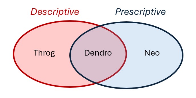
A prime use case for Dendro is inventory policy optimization: right-sizing inventory levels by changing inventory policy parameters (reorder points, reorder quantities, etc.) with the goal of balancing cost and service. Dendro's foundation in simulation minimizes the abstraction of cost accounting, service metrics, and the business rules surrounding inventory management. Dendro provides actionable inventory policy recommendations and data-driven evidence to support those changes.
Primary Focus: Determining where inventory should be positioned across the network.
Use Case: Network design decisions that include high-level inventory considerations -- such as stocking locations, target turns, and working capital trade-offs.
How It Handles Inventory:
Primary Focus: Testing and observing how specific inventory policies perform under realistic operational dynamics.
Use Case: Evaluate inventory control logic (e.g., reorder point, order quantity, order-up-to level) in a time-based simulation environment.
How It Handles Inventory:
Primary Focus: Finding better inventory policies that balance cost and service, combining Throg's simulation accuracy with an optimization engine.
Use Case: Adjust inventory policy parameters (e.g., reorder point, reorder quantity, policy type) to find configurations that deliver the best cost-service trade-offs.
How It Handles Inventory:
While this comparison highlights how each engine contributes to inventory management decisions, the specific use case covered in this article is inventory policy optimization -- using Dendro to balance total inventory carrying cost and network-level customer service (measured as quantity fill rate).
That said, Dendro's capabilities extend far beyond inventory. The same framework of input factors, output factors, and utility functions can be applied to a wide range of optimization problems -- and its utility components are not limited to just cost and service. Dendro can optimize for any measurable performance metric that matters to your business.
As stated above, a Dendro study cannot be initiated without first establishing a Throg simulation model; a Dendro project should be thought of as a simulation project with an added layer of analysis. Careful Throg model verification and validation are part of a simulation project and are therefore a prerequisite for a Dendro study. To learn how to set up a Throg simulation model, we recommend reviewing the following on-demand training content:
In addition, Throg-specific articles can be found here on the Help Center.
Throg scenario results serve as one piece of input for a Dendro run. Identification of the appropriate Throg scenario to apply Dendro to depends on the goal of the Dendro study. The network structure under which the modeler is seeking to optimize inventory policies must be represented in a Throg scenario.

Inventory policies are required to run a simulation scenario. In some cases, a modeler may not have existing inventory policies to utilize in a baseline scenario. Similarly, simulating a proposed network structure requires first setting inventory policies for new site-product combinations. To set policies, we recommend utilizing the Demand Classification utility in Cosmic Frog's Utilities module.
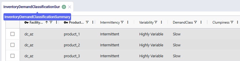

Suggested inventory policies from the Inventory Policy Data Summary output table can then be employed in the Inventory Policies input table. For the sake of testing while the Throg model is being built and verified, users may find it helpful to initially leverage simple placeholder inventory policies where policies are unknown or not yet in existence (e.g., (s,S) = (0,0)).
Note: if the modeler's goal is to set policies for a proposed network structure, it is recommended to first optimize Baseline inventory policies. This enables the modeler to compare potential performance of the existing network structure (i.e., performance under optimized policies) with performance of the proposed network structure. This is especially encouraged if the Demand Classification utility was used to set Baseline inventory policies.
Before running Dendro to optimize inventory policies, the modeler must consider
The answers to these questions will inform the design of Dendro model inputs.
Every Dendro optimization begins with a well-defined model foundation and input configuration.
This configuration tells Dendro three essential things:
Together, these define the search space and fitness criteria that drive optimization.
Dendro builds directly on your validated Throg simulation model, which serves as the environment for its optimization runs.
All Throg input tables -- facilities, customers, products, and policies -- are carried into Dendro.
For inventory-focused optimizations, the Inventory Policies input table is most critical.
It defines policy types and parameters such as reorder points and order-up-to levels. These become natural candidates for Dendro input factors.
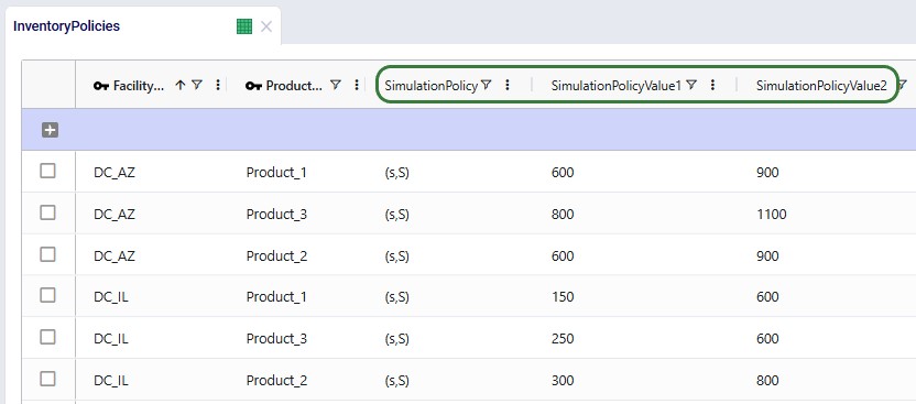
The Input Factors input table tells Dendro which parameters it can adjust during optimization. Each input factor represents a decision lever -- for instance, a reorder point or a policy type -- that Dendro will tune to seek better outcomes.
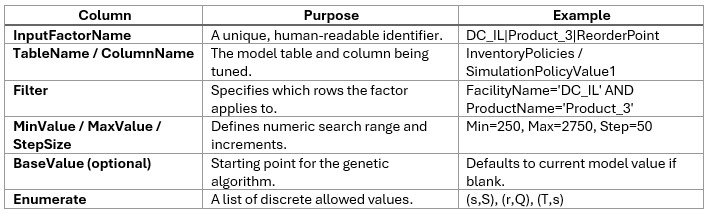
The search space defines both the breadth (how wide Dendro can explore) and the granularity (how detailed the exploration is).
The goal is a "computationally tractable search space" -- broad enough for Dendro to discover impactful alternatives but focused enough to identify patterns efficiently.
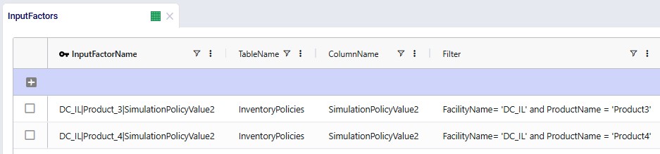

Learn all about input factors in the "Dendro: Input Factors Guide".
Once Dendro knows what it can vary, it needs to know how to judge success. The Output Factors input table defines the KPIs Dendro will use to evaluate each scenario and how they are scored.
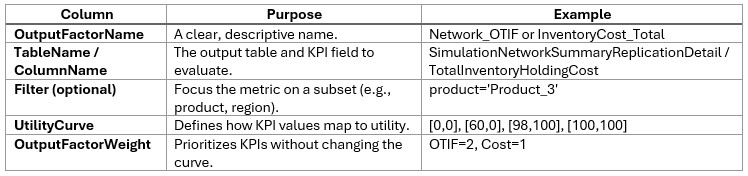
Utility curves express your business preferences:
Examples:
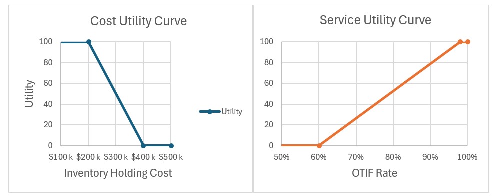
Tip: Curves should span the expected simulation range (e.g., 5th-95th percentile of early results). Dendro will stretch the utility curves if results fall outside the range, which can distort scoring.
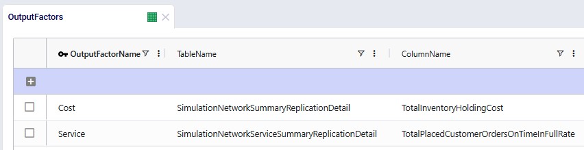
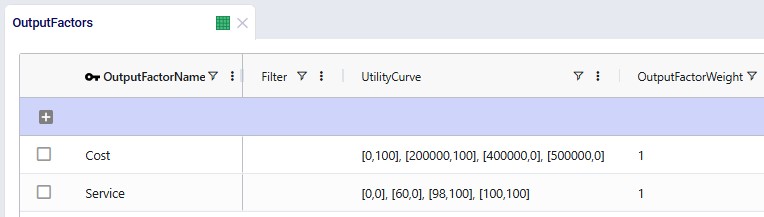
Weights dictate how much influence each KPI has in Dendro's overall fitness score calculation.
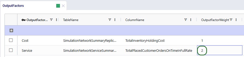
Learn more about output factors in the "Dendro: Output Factors Guide".
A well-scoped input configuration defines the playing field for Dendro's optimization.
By combining realistic input ranges, balanced KPI scoring, and robust run settings, you enable Dendro to explore intelligently finding high-performing, data-backed configurations without unnecessary computation.
Dendro is built to explore a wide range of supply chain configurations using your verified and validated Throg simulation scenario(s) as the base. Running a Dendro job is straightforward, but there are a few important steps and best practices to keep in mind to ensure smooth operation.
To get started:
INSERT INTO anura_2_8.modelrunoptions (
  datatype,
  description,
  option,
  status,
  technology,
  uidisplaycategory,
  uidisplayname,
  uidisplayorder,
  uidisplaysubcategory,
  value)
VALUES (
  'double',
  'Time limit (seconds) on individual Dendro scenarios',
  'DendroTimeout',
  'Include',
  '[DENDRO]',
  'Basic',
  'Dendro Timeout',
  '',
  '',
  '3600');
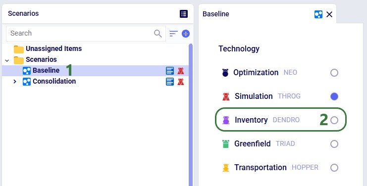
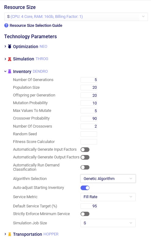
The technology parameters define how Dendro explores the solution space -- including how many scenarios to generate, how they evolve, and how long each simulation may run. As mentioned above, the default values are typically sufficient for a first run. The following are the main parameters that users may want to update in case their defaults are not suitable.
Key Settings
See also more detailed explanations of all Dendro technology parameters here.
Tuning Guidance
Use these principles to fine-tune your technology parameters:
In the course of a Dendro run, the system launches many scenarios for each generation. This is the expected behavior for the genetic algorithm.
Key tips for tracking progress:
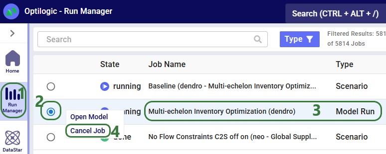
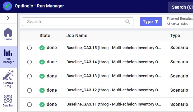
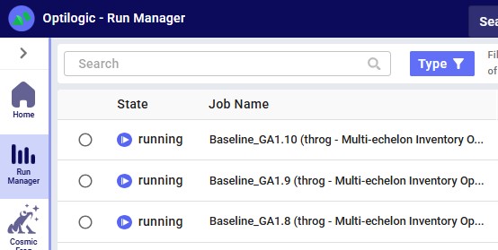
Running Dendro is as simple as selecting the engine and starting from a validated Throg model. From there, you can monitor progress, let the algorithm evolve scenarios, and apply best practices for canceling or troubleshooting runs. By following these guidelines, you ensure that Dendro can efficiently search for high-performing supply chain configurations.
To understand how the Dendro genetic algorithm works in detail, please see "Dendro: Genetic Algorithm Guide".
When a Dendro run completes, it produces a rich set of outputs that capture the results of the genetic algorithm's search. These outputs represent the different supply chain configurations that were explored, along with how each one performed according to the objectives you defined (e.g., cost, service level, or a balance of both).
Rather than giving you a single "right" answer, Dendro presents a spectrum of high-performing options. As the modeler, you use these results to evaluate trade-offs and select the scenarios that best align with your business goals.
During a run, Dendro evaluates each candidate scenario by:
Dendro records the input factors and output factors of every scenario it evaluates. However, only the top 20 highest-performing scenarios are saved as named scenarios in your model, making them easier to access and reuse.
After the run, the top 20 scenarios are automatically saved in your model. These represent the best balances of trade-offs Dendro discovered within your defined search space.
Each scenario has an overall fitness score, calculated as the weighted sum of its output factor utility values. A higher score means the scenario performed well according to the priorities you set (e.g., balancing low cost with high service).
Tip: The "best" scenario numerically may not always be the most practical operationally. Always interpret results in context.
Where to Find Key Results
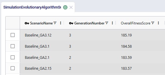
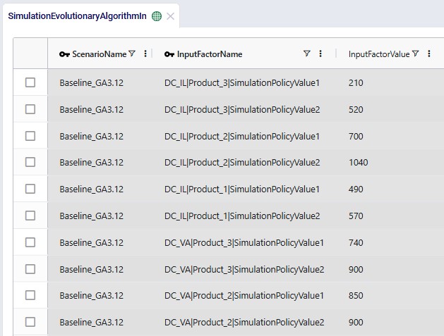

Tips for Reviewing Results
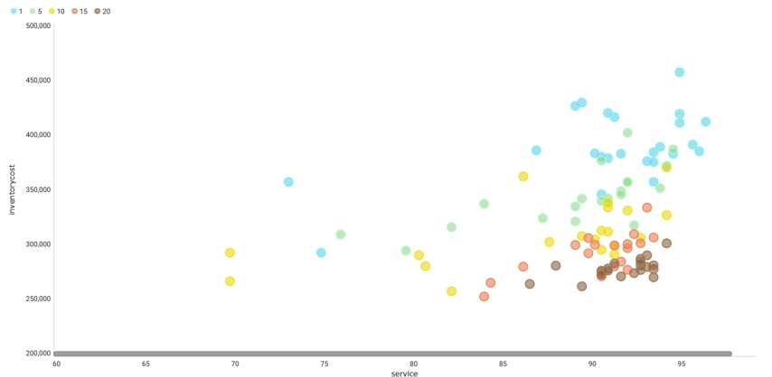
Dendro generates raw scenario outputs, but actionable recommendations come from your interpretation in the context of business goals.
In summary, Dendro does not hand you a single answer, it gives you a portfolio of high-performing options. By interpreting these scenarios in context, you can make informed decisions, balance trade-offs, and run deeper simulations where needed to guide your supply chain strategy.
You may find these links helpful, some of which have already been mentioned above:
As always, please feel free to reach out to the Optilogic Support team at support@optilogic.com in case of questions or feedback.
Dendro, Optilogic’s simulation-optimization engine, uses a sophisticated Genetic Algorithm (GA) to, for example, optimize inventory policies across your supply chain network. This guide explains how the algorithm works in business-friendly terms, helping you understand what happens when you run Dendro and how to get the best results.
The Big Picture: Dendro's Genetic Algorithm explores thousands of different inventory policy combinations, simulates each one to see how it performs, and gradually evolves toward the best possible solution - much like natural evolution produces better-adapted organisms over time.
Recommended reading prior to diving into this guide: Getting Started with Dendro, which is a higher-level overview of how Dendro works.
Genetic Algorithms are inspired by biological evolution. Just as species evolve to become better adapted to their environment through:
Dendro evolves inventory policies to become better adapted to your business objectives through:
Traditional optimization methods struggle with inventory networks due to:
Genetic Algorithms excel at this type of problem because they:
Dendro's implementation uses three fundamental elements: chromosomes, genes, and fitness score.
A chromosome represents one complete set of inventory policies for your entire supply chain.
Example Chromosome:
Each chromosome is essentially a complete "proposal" for how to manage inventory across your network.
Each gene within a chromosome represents the policy for one facility-product combination.
Example Gene:
Genes can mutate (change their values) to explore different policy settings.
The fitness score measures how good a chromosome is - combining costs, service levels, and other objectives.
Higher scores are better - Dendro displays scores where better solutions have higher values.
A fitness score might combine:
Whenever the below refers to an option, this is a model run option that can be set in the Dendro section of the Technology Parameters on the right-hand side of the Run Settings screen that comes up after a user clicks on the green Run button in Cosmic Frog.
What happens: Dendro creates the initial population of chromosomes (policy combinations).
Implementation details:
Business perspective: Think of this as Dendro assembling a diverse team of proposals. The first proposal is "keep doing what we are doing", while the others explore variations like "increase safety stock by 10%", "reduce order quantities", etc.
Each generation follows the same four-step cycle:
What happens: Each chromosome is evaluated by:
Implementation details:
Business perspective: Dendro tests each proposal by running it through a realistic simulation of your supply chain over time. It is like running a pilot program for each policy combination to see what would actually happen - but virtually, so you can test thousands of options without risk.
Typical duration:
What happens: Dendro ranks all chromosomes by fitness score and selects the best ones to continue to the next generation.
Implementation details:
Business perspective: After testing all proposals, Dendro keeps the most promising ones and discards the poor performers. This is like a review committee keeping the best ideas and dropping the ones that do not work well.
Example:
Generation 5 Results (20 chromosomes evaluated):
What happens: Dendro creates new chromosomes by combining parts of two successful parent chromosomes.
Implementation details:
Business perspective: Dendro creates new proposals by combining the best parts of successful proposals. If one policy set works well for East Coast facilities and another works well for high-volume products, crossover might create a policy that combines both successful approaches.
Example with 1-Point Crossover:
Parent 1: [Gene_A1, Gene_A2, Gene_A3, Gene_A4, Gene_A5]
Parent 2: [Gene_B1, Gene_B2, Gene_B3, Gene_B4, Gene_B5]
↑ Crossover point
Offspring 1: [Gene_A1, Gene_A2, Gene_A3 | Gene_B4, Gene_B5]
Offspring 2: [Gene_B1, Gene_B2, Gene_B3 | Gene_A4, Gene_A5]
When crossover is most effective:
What happens: Dendro randomly adjusts policy values in the new chromosomes to explore variations.
Implementation details:
Business perspective: Dendro introduces controlled randomness to explore new options. Even the best current policies might not be optimal, so mutation ensures the algorithm does not get stuck. It is like saying "this policy works well at 500 units, but let's try 525 and 475 too".
Example mutations:
Original Gene: Reorder Point = 500, Order-Up-To = 1000
Mutated Gene: Reorder Point = 525, Order-Up-To = 1050
Mutation strategies:
Input factors define what Dendro can change. They are the "variables" in your optimization problem. They can be specified in the Input Factors input table in your Cosmic Frog model.
Common input factors:
How they work in chromosomes: Each input factor becomes a position in the chromosome. Dendro explores different values for each position.
Example: If you have 50 facility-product combinations to optimize, and each has two policy values (reorder point and order-up-to), your chromosome has 50 genes, each with 2 values = 100 total parameters being optimized.
Input factors are covered in detail in the Dendro: Input Factors Guide.
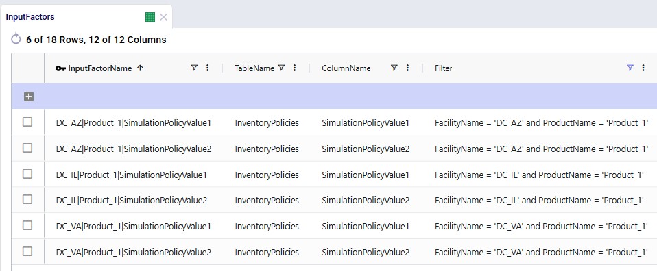
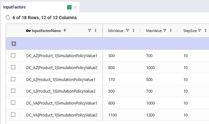
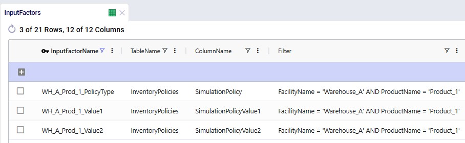
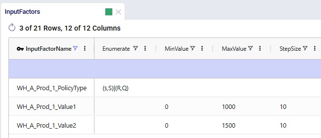
The following 2 screenshots show 6 records in an Input Factors input table in Cosmic Frog. Both simulation policy values for Product_1 at 3 different DCs are specified in these records:
Output factors define what Dendro tries to minimize. They are the "objectives" in your optimization problem. Output factors can be set in the Output Factors input table.
Common output factors:
How they combine - each output factor has a:
The Dendro: Output Factors Guide covers output factors in more detail.
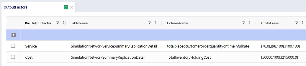
The following screenshot shows an output factors table containing 2 output factors, one measuring service and the other cost:
Utility curves convert simulation outputs into comparable fitness scores.
Why we need them:
How they work:
Example:
Holding Cost Utility Curve:
Business benefit: Utility curves let you define what "good" and "bad" mean for each metric. They translate apples-and-oranges metrics into a single comparable score.
The overall fitness score is the weighted sum of all output factors.
Formula:
Fitness Score = Σ(Weighted Score for each Output Factor)
Where for each factor:
Weighted Score = (Normalized Score from Utility Curve) × (Factor Weight)
Higher is better - Better solutions receive higher fitness scores.
Example calculation:
Output Factors:
1. Holding Cost: $75,000 → Raw Score 75 → Weighted 22.5 (weight 30%)
2. Transport Cost: $40,000 → Raw Score 60 → Weighted 15.0 (weight 25%)
3. Stockout Penalty: $10,000 → Raw Score 80 → Weighted 20.0 (weight 25%)
4. Service Level: 96% → Raw Score 90 → Weighted 18.0 (weight 20%)
Overall Fitness = 22.5 + 15.0 + 20.0 + 18.0 = 75.5 points
Important note: Scores are recalculated when new min/max values are discovered to ensure fair comparison across all generations.
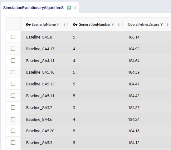
After a Dendro run completes, the fitness scores of all scenarios (=chromosomes) of all generations can be found in the Simulation Evolutionary Algorithm Summary output table (showing the top 10 records here with the highest overall fitness scores):
The challenge: Early in the optimization, Dendro does not know what the best and worst possible values are for each metric. As it explores, it might find:
The solution: Dendro dynamically rescales utility curves when new extremes are discovered.
What happens:
Business perspective: This ensures that a solution that looked "good" in Generation 2 is not unfairly favored if better solutions are discovered later. Everyone is judged by the same standard.
Keeping the best results:
Small population, many generations:
Characteristics:
Large population, fewer generations:
Characteristics:
Balanced approach (recommended):
High mutation (100% probability):
Low mutation (30-50% probability):
Single-point crossover (default):
Points To Crossover = 1
Multi-point crossover:
Points To Crossover = 2 or more
When to disable crossover:
Key indicators of healthy optimization:
The Simulation Evolutionary Algorithm Summary output table can be used to assess the above 2 points as it contains the fitness scores of all scenarios (=chromosomes) that were run for all generations. See an example screenshot of this table further above in the Fitness Score Calculation section.
This last point can be assessed by reviewing the logs of the base scenario used for the Dendro run.
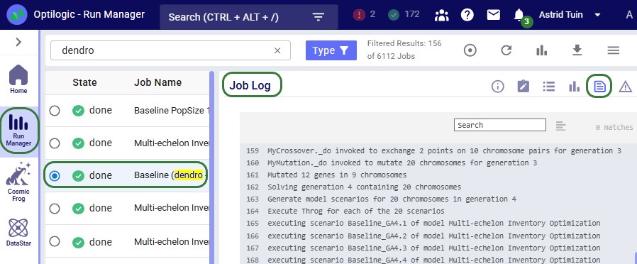
Logging output: Dendro logs key events. These can be found in the Run Manager application, which is another application on the Optilogic platform. The Job Log of the base scenario that Dendro is run on contains quite a lot of detailed on events, such as:
This screenshot shows part of a Job Log for a Dendro run:
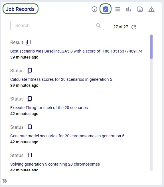
The Job Records log, which can be accessed by clicking on the second icon in the row of icons at the top right of the logs provides a higher level summary of the Dendro run, just calling out the main events:
The GA excels in following situations:
The mechanism: Dendro automatically detects and eliminates duplicate chromosomes.
How it works:
Business benefit: Ensures computational resources are used efficiently - never simulating the same policy combination twice.
Challenge: Each chromosome generates a simulation scenario with potentially gigabytes of output data.
Solution:
Business benefit: You can analyze the best solutions in detail without storing data for thousands of unsuccessful experiments.
Network:
Configuration:
Process:
Generation 1:
Generations 2-10:
Generations 11-15:
Generations 16-20:
Results:
Dendro's Genetic Algorithm is a powerful, flexible optimization engine that:
By understanding how the algorithm works, you can:
The GA is not magic – it is a systematic, intelligent search process. Like any tool, it works best when used thoughtfully and configured appropriately for your specific situation.
You may find these links helpful, some of which have already been mentioned above:
Please do not hesitate to contact the Optilogic Support team on support@optilogic.com for any questions or feedback.
Input factors are at the heart of Dendro optimization - they define what Dendro can change to improve your supply chain performance. Think of input factors as the "knobs" Dendro can turn to find better inventory policies.
Key concepts:
This guide explains how to configure input factors to give Dendro the right level of control over your inventory policies. These can be specified in the Input Factors input table in Cosmic Frog.
Recommended reading prior to diving into this guide: Getting Started with Dendro, a high-level overview of how Dendro works, and Dendro: Genetic Algorithm Guide which explains the inner workings of Dendro in more detail.
An input factor tells Dendro's Genetic Algorithm:
Dendro explores these decisions systematically across your entire network to find the optimal combination.
Dendro supports three types of input factors, each suited for different kinds of optimization variables. These are all specified on the Input Factors input table, see also "The Input Factors Table" section further below.
What they are: Numeric values that can vary within a minimum and maximum range.
Best for:
Configuration fields:
InputFactorName: WH_A_Prod_1_ReorderPoint TableName: InventoryPolicies ColumnName: SimulationPolicyValue1 Filter: FacilityName='Warehouse A' AND ProductName='Product 1' MinValue: 100 MaxValue: 1000 StepSize: 10 BaseValue: 500 How it works:
Example:
Chromosome 1 (baseline): 500 Chromosome 2 (random): 730 Chromosome 3 (random): 220 Chromosome 4 (mutated from 2): 740 (increased by one step) What they are: Values selected from a predefined list of discrete options.
Best for:
Configuration fields:
InputFactorName: DC_Policy_Type TableName: InventoryPolicies ColumnName: SimulationPolicy Filter: FacilityName='Distribution Center' Enumerate: (s,S)|(R,Q)|(T,S) BaseValue: (s,S) How it works:
Example:
Chromosome 1 (baseline): (s,S) Chromosome 2 (random): (R,Q) Chromosome 3 (random): (T,S) Chromosome 4 (mutated from 2): (s,S) (switched from R,Q) What they are: Grouped input factors that manage related inventory policy parameters together as a coordinated set.
Best for:
How they work:
Example configuration:
Factor 1: InputFactorName: WH_A_Prod_1_PolicyType TableName: InventoryPolicies ColumnName: SimulationPolicy Filter: FacilityName='Warehouse A' AND ProductName='Product 1' Enumerate: (s,S)|(R,Q) Factor 2: InputFactorName: WH_A_Prod_1_Value1 TableName: InventoryPolicies ColumnName: SimulationPolicyValue1 Filter: FacilityName='Warehouse A' AND ProductName='Product 1' MinValue: 0 MaxValue: 1000 StepSize: 10 Factor 3: InputFactorName: WH_A_Prod_1_Value2 TableName: InventoryPolicies ColumnName: SimulationPolicyValue2 Filter: FacilityName='Warehouse A' AND ProductName='Product 1' MinValue: 0 MaxValue: 1500 StepSize: 10 Automatic policy conversion: When policy type changes from (R,Q) to (s,S):
When changing from (s,S) to (R,Q):
Input factors are configured in the Input Factors input table with the following columns:
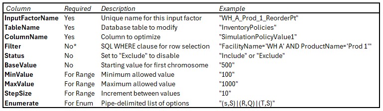
*Filter is required for inventory policy input factors to identify the specific facility-product combination.
The following 2 screenshots show the Input Factors table in Cosmic Frog. It contains 3 records which are set up the same as the example in the "Inventory Policy Sets (Advanced)" section above:
Optimize the reorder point for a single facility-product:
InputFactorName: Seattle_Widget_ReorderPoint TableName: InventoryPolicies ColumnName: SimulationPolicyValue1 Filter: FacilityName='Seattle DC' AND ProductName='Widget A' MinValue: 200 MaxValue: 800 StepSize: 20 BaseValue: 500 Status: Include Result: Dendro will explore reorder points from 200 to 800 in steps of 20 (200, 220, 240, ..., 800).
Optimize order quantity with small increments:
InputFactorName: Boston_Gadget_OrderQty TableName: InventoryPolicies ColumnName: SimulationPolicyValue2 Filter: FacilityName='Boston WH' AND ProductName='Gadget B' MinValue: 50 MaxValue: 500 StepSize: 5 BaseValue: 200 Status: Include Result: Dendro will explore 91 different values (50, 55, 60, ..., 500).
Let Dendro choose between different inventory policies:
InputFactorName: Chicago_Part_PolicyType TableName: InventoryPolicies ColumnName: SimulationPolicy Filter: FacilityName='Chicago Plant' AND ProductName='Part C' Enumerate: (s,S)|(R,Q)|(T,S) BaseValue: (s,S) Status: Include Result: Dendro will test (s,S), (R,Q), and (T,S) policies to see which performs best.
Optimize both policy type and parameters:
Policy Type InputFactorName: LA_Motor_PolicyType TableName: InventoryPolicies ColumnName: SimulationPolicy Filter: FacilityName='LA Warehouse' AND ProductName='Motor D' Enumerate: (s,S)|(R,Q) BaseValue: (s,S) Parameter 1 (reorder point or 's') InputFactorName: LA_Motor_Value1 TableName: InventoryPolicies ColumnName: SimulationPolicyValue1 Filter: FacilityName='LA Warehouse' AND ProductName='Motor D' MinValue: 0 MaxValue: 500 StepSize: 10 BaseValue: 100 Parameter 2 (order-up-to or order quantity) InputFactorName: LA_Motor_Value2 TableName: InventoryPolicies ColumnName: SimulationPolicyValue2 Filter: FacilityName='LA Warehouse' AND ProductName='Motor D' MinValue: 0 MaxValue: 800 StepSize: 10 BaseValue: 300 Result: Dendro will:
The most common input factors for inventory optimization target these columns in the Inventory Policies input table:

Example:
Input Factors:
[0] WH_A_Prod_1_ReorderPoint (Range: 100-1000, Step: 10, Base: 500) [1] WH_A_Prod_1_ReorderPoint (Range: 200-800, Step: 20, Base: 400) [2] WH_A_Prod_1_PolicyType (Enum: (s,S)|(R,Q), Base: (s,S))Results in:
Chromosome 1 (baseline): [500, 400, 0] (0 = first enum value = (s,S)) Chromosome 2 (random): [730, 560, 1] (1 = second enum value = (R,Q)) Chromosome 3 (random): [220, 640, 0] (0 = first enum value = (s,S))When Dendro mutates a chromosome, it changes one or more input factor values:
For Range factors:
For Enumeration factors:
Example mutation:
Original: [500, 400, 0] Mutated: [500, 420, 0] (Position 1 changed: 400 to 420) When Dendro creates a scenario to simulate using the Throg engine:
Result: Each chromosome becomes a complete, runnable supply chain scenario with its specific inventory policy settings.
When turned on, the Automatically Generate Input Factors option (a model run option in the Dendro section of the Technology Parameters) automatically creates input factor configurations based on your inventory policies and service targets.
When to use:
How it works:
The automatic builder uses intelligent rules to set min/max ranges based on current values and service performance:
MinValue: 0 MaxValue: value + 5 (or adjusted based on service) StepSize: 1 Rationale: Small values need fine-grained control and room to explore modest increases.
MinValue: max(1, rounded_value - 15) MaxValue: rounded_value + 15 StepSize: 5 Values are rounded to base 5
Rationale: Medium values can use larger steps (5) while still providing good resolution.
MinValue: max(1, rounded_value - 50) MaxValue: rounded_value + 50 StepSize: 10 Values are rounded to base 10
Rationale: Larger inventories need wider exploration ranges with proportionally larger steps.
MinValue: max(1, rounded_value - 200) MaxValue: rounded_value + 200 StepSize: 20 Values are rounded to base 20
Rationale: Very large inventories benefit from broad exploration with coarse granularity.
The builder adjusts ranges based on current service performance:
When fill rate < target service level: The ratio = target_service / current_fill_rate is used to expand the maximum:
MaxValue = max(value + buffer, ratio * value)
Example:
When fill rate => target service level: The builder is more conservative, allowing exploration below current value:
MaxValue = min(value + buffer, quantity_bounds)
Rationale: If service is already good, there may be opportunity to reduce inventory without harming service.
When fill rate <= 85% (poor service): MinValue is set to current value - does not explore lower values that would worsen service further.
For each inventory policy, the automatic generator typically creates:
Result: A complete Input Factors table ready for Dendro optimization.
Too narrow:
MinValue: 490 MaxValue: 510 StepSize: 1 Problem: Dendro cannot explore significantly different solutions. Only 21 values to test.
Too wide:
MinValue: 0 MaxValue: 100000 StepSize: 1 Problem: 100,000 possible values means Dendro will likely miss the optimal value in the haystack.
Just right:
MinValue: 200 MaxValue: 800 StepSize: 20 Why: Reasonable range around current value (500), coarse enough for efficient exploration (31 values), fine enough for precision.
Rule of thumb: Step size should be 1-5% of the expected optimal value.
For value of approximately 100:
For value of approximately 1000:
Why it matters:
Bad:
MinValue: 100 MaxValue: 1000 StepSize: 40 Problem: (1000-100) / 40 = 22 remainder 20; the max might not be reachable exactly.
Good:
MinValue: 100 MaxValue: 1000 StepSize: 30Check: (1000-100) / 30 = 30 remainder 0; the max can be reached exactly.
Dendro automatically adjusts MaxValue if needed to ensure even division.
Best practice: Set BaseValue to your current policy value.
Why:
When BaseValue is null:
For inventory policies, always configure factors for the same facility-product together:
Good - Coordinated filters:
All three factors have identical FilterWH_A_Prod_1_PolicyType Filter: FacilityName='WH A' AND ProductName='Prod 1' WH_A_Prod_1_Value1 Filter: FacilityName='WH A' AND ProductName='Prod 1' WH_A_Prod_1_Value2 Filter: FacilityName='WH A' AND ProductName='Prod 1' Bad - Mismatched filters:
WH_A_Prod_1_PolicyType Filter: FacilityName='WH A' AND ProductName='Prod 1' WH_A_Prod_1_Value1 Filter: FacilityName='WH A' AND ProductName='Prod 1' WH_A_AllProds_Value2 Filter: FacilityName='WH A' # WRONG - does not match! Why: Dendro groups factors by filter. Mismatched filters create separate uncoordinated genes.
Guideline: More input factors = larger search space = longer optimization
Example calculation:
Search space size: 50^200 = enormous!
Best practice:
Use the Status column: Set Status = 'Exclude' for factors you want to temporarily disable without deleting.
Common mistakes:
Wrong - Missing quotes:
Filter: FacilityName=Warehouse A AND ProductName=Widget
Correct - Proper quotes:
Filter: FacilityName='Warehouse A' AND ProductName='Widget'
Wrong - Incorrect column names:
Filter: Facility='WH A' AND Product='Widget'
Correct - Match actual table column names:
Filter: FacilityName='WH A' AND ProductName='Widget'
Testing tip: Run your filter as a SQL WHERE clause to verify it returns exactly one row (you can use the SQL Editor application on the Optilogic platform for this):
SELECT * FROM InventoryPolicies
WHERE FacilityName='WH A' AND ProductName='Widget';Goal: Keep current policy types and order quantities; optimize reorder points only.
Configuration:
For each facility-product:
InputFactorName: {Facility}_{Product}_ReorderPt TableName: InventoryPolicies ColumnName: SimulationPolicyValue1 Filter: FacilityName='{Facility}' AND ProductName='{Product}' MinValue: [calculated] MaxValue: [calculated] StepSize: [appropriate for value scale] BaseValue: [current value] Result: Dendro explores different reorder points while keeping other policy parameters fixed.
Goal: Let Dendro choose policy types and all parameters.
Configuration:
For each facility-product:
Policy typeInputFactorName: {Facility}_{Product}_Policy TableName: InventoryPolicies ColumnName: SimulationPolicy Filter: FacilityName='{Facility}' AND ProductName='{Product}' Enumerate: (s,S)|(R,Q)Parameter 1 InputFactorName: {Facility}_{Product}_Value1 TableName: InventoryPolicies ColumnName: SimulationPolicyValue1 Filter: FacilityName='{Facility}' AND ProductName='{Product}' [Range configuration] Parameter 2 InputFactorName: {Facility}_{Product}_Value2 TableName: InventoryPolicies ColumnName: SimulationPolicyValue2 Filter: FacilityName='{Facility}' AND ProductName='{Product}' [Range configuration] Result: Maximum flexibility - Dendro explores different policy types and parameter values.
Goal: Optimize top 20% of items by revenue; leave others unchanged.
Approach:
SQL example for selective generation - Create Input Factors for top revenue items only:
INSERT INTO InputFactors (...)
SELECT ... FROM InventoryPolicies ip
JOIN ProductRevenue pr ON ip.ProductName = pr.ProductName
WHERE pr.AnnualRevenue > [threshold]
Result: Focused optimization on items that matter most, faster runtime.
Goal: Use wider ranges for variable-demand products, tighter for stable products.
Configuration:
Stable, predictable products:
MinValue: current_value * 0.8 MaxValue: current_value * 1.2 StepSize: small (fine control) Variable, unpredictable products:
MinValue: current_value * 0.5 MaxValue: current_value * 2.0 StepSize: larger (broader exploration) Result: Appropriate exploration ranges based on demand variability.
Symptom: During loading, you see "no matching inventory policy" in the Job Log.
Cause: The Filter does not match any row in the InventoryPolicies table.
Solutions:
SELECT * FROM InventoryPolicies WHERE [your filter]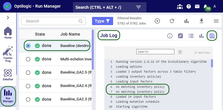
Symptom: Multiple separate genes instead of one coordinated policy set.
Cause: Filters do not match exactly across related factors.
Example problem:
Factor 1 Filter: FacilityName='WH A' AND ProductName='Widget' Factor 2 Filter: FacilityName='WH A' and ProductName='Widget' # lowercase 'and'! Solution: Ensure identical filter text across all factors for the same facility-product.
Symptom: Dendro tests impractical inventory levels (too high or too low).
Cause: Min/Max ranges too wide or poorly set.
Solutions:
Symptom: Fitness scores are not getting better across generations.
Possible causes:
Cause 1: Ranges too narrow
Cause 2: Step size too coarse
Cause 3: Wrong factors optimized
Cause 4: Conflicting objectives
Overall Fitness Scores can be assessed in the Simulation Evolutionary Algorithm Summary output table after a Dendro run has completed, while scores of individual output factors can be reviewed in the Simulation Evolutionary Algorithm Output Factor Report output table:
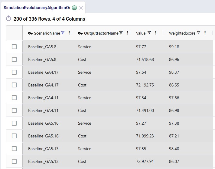
Symptom: Warnings or errors about order-up-to levels below reorder points.
Cause: Ranges configured without considering logical constraints.
Solution: Dendro handles this automatically through special mutation logic, but you can help by:
Note: Dendro automatically enforces S => s during gene creation and mutation.
Input factors are the foundation of Dendro optimization:
Key takeaways:
Well-configured input factors give Dendro the right level of control to find optimal solutions efficiently. Too much freedom creates an intractably large search space; too little prevents discovering improvements. The art is finding the right balance for your specific supply chain.
You may find these links helpful, some of which have already been mentioned above:
Please do not hesitate to contact the Optilogic Support team on support@optilogic.com for any questions or feedback.
Output factors define what Dendro tries to optimize - they are your business objectives translated into measurable metrics. While input factors control what can change, output factors determine what "better" means.
Key concepts:
This guide explains how to configure output factors to align Dendro's optimization with your business goals. These can be specified in the Output Factors input table in Cosmic Frog models.
Recommended reading prior to diving into this guide: Getting Started with Dendro, a high-level overview of how Dendro works, and Dendro: Genetic Algorithm Guide which explains the inner workings of Dendro in more detail.
An output factor tells Dendro's genetic algorithm:
Imagine you are evaluating employee performance:
Dendro uses the same approach to evaluate inventory policy combinations across your supply chain.
Output factors are configured in the Output Factors input table with the following columns:
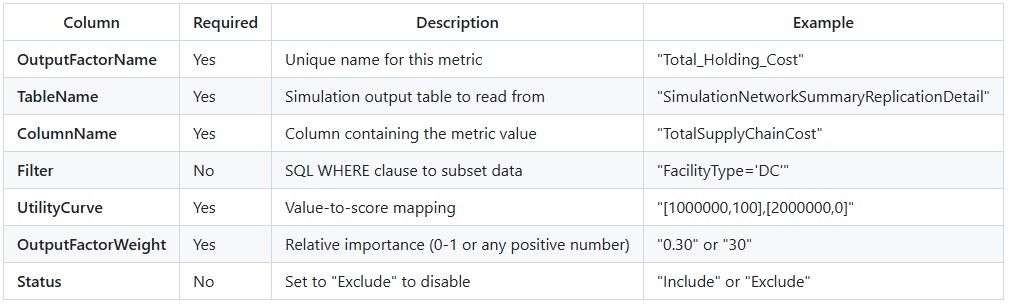
Minimize overall supply chain costs:
OutputFactorName: TotalCost TableName: SimulationNetworkSummaryReplicationDetail ColumnName: TotalSupplyChainCost Filter: (leave empty for all data)UtilityCurve: [1500000,100],[2000000,0]OutputFactorWeight: 0.40 Status: Include Interpretation:
Maximize service level performance:
OutputFactorName: ServiceLevel TableName: SimulationNetworkServiceSummaryReplicationDetailColumnName: TotalPlacedCustomerOrderQuantityOnTimeInFullRate Filter: (leave empty) UtilityCurve: [0,0],[85,10],[95,99],[100,100]OutputFactorWeight: 0.35 Status: Include Interpretation:
Focus on inventory costs at distribution centers only:
OutputFactorName: DC_HoldingCost TableName: SimulationFacilityCostSummaryReplicationDetail ColumnName: InventoryHoldingCost Filter: FacilityType='DC' UtilityCurve: [50000,100],[150000,0]OutputFactorWeight: 0.25 Status: Include Interpretation:
The following 2 screenshots show the Output Factors input table in Cosmic Frog; it contains 3 rows which represent the 3 examples above:
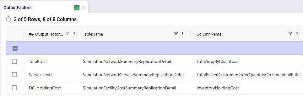
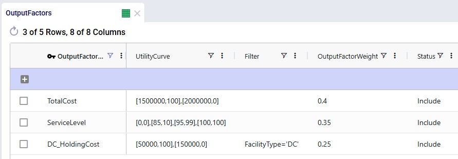
A utility curve translates raw metric values (like dollars or percentages) into standardized quality scores (0-100 points). It answers the question: "How good is this value?".
Format:[value1,score1],[value2,score2],[value3,score3],...
Each [value,score] pair defines a point on the curve:
Dendro connects these points with straight lines to create a piecewise linear curve.
[1000,100],[2000,0]
Meaning:
Visualization:
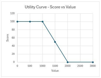
Best for:
[50,0],[100,50],[150,100]
Meaning:
Visualization:
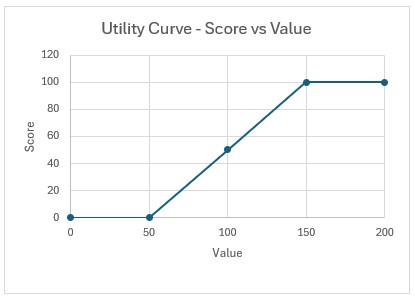
Best for:
[0,0],[85,10],[95,99],[100,100]
Meaning:
Characteristics:
Visualization:
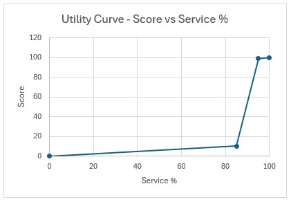
Best for:
The challenge: Early in optimization, Dendro does not know what the best and worst possible values are.
The solution: Utility curves automatically expand when new extremes are discovered.
Example scenario:
Generation 1:
[1800000,100],[2200000,0]Generation 5:
[1600000,100],[2200000,0]Why it matters:
When rescaling occurs:
Weights determine how much each output factor contributes to the overall fitness score.
Common approaches:
Total Cost: Weight = 0.40 (40%) Service Level: Weight = 0.35 (35%) Inventory Value: Weight = 0.25 (25%) Total = 1.00 (100%) Advantage: Easy to understand - directly represents percentage contribution.
Total Cost: Weight = 40 Service Level: Weight = 35 Inventory Value: Weight = 25 Total = 100 (but could be any sum) Advantage: Can use any convenient scale; Dendro handles normalization.
Critical Factor: Weight = 10 Important Factor: Weight = 5 Secondary Factor: Weight = 2 Minor Factor: Weight = 1 Advantage: Emphasizes relative priorities clearly.
Example calculation:
Output Factors:
Holding Cost: Raw value = $80,000 → Utility score = 60 → Weight = 0.40 Service Level: Raw value = 94% → Utility score = 85 → Weight = 0.35 Transport Cost: Raw value = $45,000 → Utility score = 70 → Weight = 0.25 Weighted Contributions:
Holding Cost: 60 × 0.40 = 24.0 pointsService Level: 85 × 0.35 = 29.75 points Transport Cost: 70 × 0.25 = 17.5 points Overall Fitness Score: 24.0 + 29.75 + 17.5 = 71.25 points
Higher fitness scores are better in Dendro
The fitness calculation adds these weighted scores, so the formula is:
Fitness = 24.0 + 29.75 + 17.5 = 71.25
Balanced approach:
Cost factors (total): 50% Service factors (total): 50% Equal priority to cost reduction and service achievement.
Cost-focused approach:
Cost factors (total): 70% Service factors (total): 30% Emphasizes cost minimization; willing to accept moderate service levels.
Service-focused approach:
Cost factors (total): 30% Service factors (total): 70% Prioritizes customer service; cost is secondary.
Multi-objective balanced:
Holding cost: 25% Transport cost: 25% Service level: 25% Inventory turns: 25% Equal consideration to multiple objectives.
For each output factor, Dendro reads the metric value from the simulation results:
Factor 1 (Total Cost): Reads TotalSupplyChainCost → $1,750,000 Factor 2 (Service Level): Reads OnTimeInFullRate → 92% Factor 3 (Holding Cost): Reads InventoryHoldingCost → $320,000 Each value is mapped to a raw score using its utility curve:
Factor 1: $1,750,000 → Utility curve [1500000,100],[2000000,0]Interpolation: (1,750,000 - 1,500,000) / (2,000,000 - 1,500,000) = 0.5 Raw score: 100 - (0.5 × 100) = 50 Factor 2: 92% → Utility curve [0,0],[85,10],[95,99],[100,100]Falls between 85 and 95: Interpolate Raw score: 10 + ((92-85)/(95-85)) × (99-10) = 10 + 62.3 = 72.3Factor 3: $320,000 → Utility curve [200000,100],[400000,0]Interpolation: (320,000 - 200,000) / (400,000 - 200,000) = 0.6Raw score: 100 - (0.6 × 100) = 40 Utility scores are scaled to a 0-100 range based on the min/max scores in the curve:
If all curves use 0-100 range → No additional scaling neededScores are already normalized: 50, 72.3, 40 Multiply each normalized score by its weight:
Factor 1: 50 × 0.40 = 20.0 Factor 2: 72.3 × 0.35 = 25.3 Factor 3: 40 × 0.25 = 10.0 Combine all weighted scores:
Overall score = 20.0 + 25.3 + 10.0 = 55.3
Chromosome A:
Total Cost: $1,600,000 → Score 80 → Weighted 32.0 Service: 96% → Score 100 → Weighted 35.0 Holding: $280,000 → Score 60 → Weighted 15.0 Total: 82.0 Chromosome B:
Total Cost: $1,750,000 → Score 50 → Weighted 20.0 Service: 92% → Score 72 → Weighted 25.2 Holding: $320,000 → Score 40 → Weighted 10.0 Total: 55.2 Result: Chromosome A (fitness score of 82.0) is better than Chromosome B (fitness score of 55.2).
Chromosome A achieves better performance across all metrics, resulting in a higher fitness score.
In Cosmic Frog, the Overall Fitness Scores of all scenarios (=chromosomes) run can be assessed in the Simulation Evolutionary Algorithm Summary output table after a Dendro run has completed. Scores of individual output factors can be reviewed in the Simulation Evolutionary Algorithm Output Factor Report output table:
The Automatically Generate Output Factors option automatically creates standard output factor configurations based on your target service levels and baseline simulation results. This option can be set in the Dendro section of the Technology Parameters.
When to use:
What it creates:
Step 1: Run baseline simulation Execute your current inventory policies to measure actual cost.
Step 2: Establish boundaries
Baseline Cost: $1,800,000 Left Boundary (best): 75% of baseline = $1,350,000 Right Boundary (worst): 110% of baseline = $1,980,000 Step 3: Create utility curve
UtilityCurve: [1350000,100],[1980000,0]
Interpretation:
Step 4: Set weight
OutputFactorWeight: 1 (50% when combined with service factor)
Step 1: Use configured service targets
DefaultTargetService: 95% LowService: 85% Step 2: Create multi-point utility curve
UtilityCurve: [0,0],[85,10],[95,99],[100,100]
Interpretation:
Design rationale:
Step 3: Set weight
OutputFactorWeight: 1 (50% when combined with cost factor)
OutputFactors Table:
Row 1: OutputFactorName: Cost TableName: SimulationNetworkSummaryReplicationDetailColumnName: TotalSupplyChainCost Filter: NULL UtilityCurve: [1350000,100],[1980000,0]OutputFactorWeight: 1 Status: Include Row 2: OutputFactorName: Service TableName: SimulationNetworkServiceSummaryReplicationDetailColumnName: TotalPlacedCustomerOrderQuantityOnTimeInFullRateFilter: NULL UtilityCurve: [0,0],[85,10],[95,99],[100,100]OutputFactorWeight: 1 Status: Include Optimization behavior: Dendro will seek policies that:
Goal: Find the lowest-cost inventory policies without service constraints.
Setup:
OutputFactorName: TotalCost TableName: SimulationNetworkSummaryReplicationDetailColumnName: TotalSupplyChainCost UtilityCurve: [1000000,100],[3000000,0]OutputFactorWeight: 1.0 Result: Dendro minimizes cost aggressively; service may suffer.
When to use:
Goal: Maximize service while preventing excessive cost increases.
Setup:
Factor 1 - Service (Primary): OutputFactorName: Service TableName: SimulationNetworkSummaryReplicationDetailColumnName: OnTimeInFullRate UtilityCurve: [90,0],[95,50],[98,99],[100,100]OutputFactorWeight: 0.70 Factor 2 - Cost (Constraint):OutputFactorName: CostLimit TableName: SimulationNetworkSummaryReplicationDetailColumnName: TotalSupplyChainCost UtilityCurve: [1500000,100],[2000000,50],[2500000,0]OutputFactorWeight: 0.30 Result: Dendro prioritizes service but penalizes solutions exceeding cost thresholds.
When to use:
Goal: Optimize multiple objectives with balanced priorities.
Setup:
Factor 1 - Holding Cost: OutputFactorName: HoldingCost TableName: SimulationNetworkSummaryReplicationDetailColumnName: InventoryHoldingCost UtilityCurve: [200000,100],[500000,0]OutputFactorWeight: 0.25 Factor 2 - Transport Cost: OutputFactorName: TransportCostTableName: SimulationNetworkSummaryReplicationDetailColumnName: TransportationCost UtilityCurve: [300000,100],[600000,0]OutputFactorWeight: 0.25 Factor 3 - Service Level: OutputFactorName: Service TableName: SimulationNetworkSummaryReplicationDetailColumnName: FillRate UtilityCurve: [85,0],[95,99],[100,100]OutputFactorWeight: 0.30 Factor 4 - Inventory Turns: OutputFactorName: InventoryTurnsTableName: SimulationNetworkSummaryReplicationDetailColumnName: InventoryTurns UtilityCurve: [2,0],[6,50],[12,100]OutputFactorWeight: 0.20 Result: Dendro finds well-rounded solutions balancing cost, service, and efficiency.
When to use:
Goal: Different service targets for different regions.
Setup:
Factor 1 - Premium Region Service: OutputFactorName: Premium_Service TableName: SimulationNetworkSummaryReplicationDetailColumnName: FillRate Filter: Region='Premium' UtilityCurve: [92,0],[98,99],[100,100]OutputFactorWeight: 0.40 Factor 2 - Standard Region Service: OutputFactorName: Standard_Service TableName: SimulationNetworkSummaryReplicationDetailColumnName: FillRate Filter: Region='Standard' UtilityCurve: [85,0],[92,99],[100,100]OutputFactorWeight: 0.30 Factor 3 - Overall Cost: OutputFactorName: TotalCost TableName: SimulationNetworkSummaryReplicationDetailColumnName: TotalSupplyChainCost UtilityCurve: [2000000,100],[3000000,0]OutputFactorWeight: 0.30 Result: Premium regions get higher service targets; standard regions have lower thresholds.
When to use:
Some output tables contain multiple rows per scenario (e.g., one row per facility or product). Dendro combines these into a single metric value by using a straight average calculation. More options will be added in future releases.
How it works: Calculates the arithmetic mean of all matching rows.
SQL equivalent:
SELECT AVG(ColumnName)
FROM TableName
WHERE ScenarioName = 'Gen3_Chr5' AND [Filter]
Example:
Facility A holding cost: $80,000 Facility B holding cost: $120,000 Facility C holding cost: $100,000 SimpleAverage: ($80,000 + $120,000 + $100,000) / 3 = $100,000 Best for:
Do not use:
[0,0],[10,5],[20,15],[30,28],[40,45],[50,65],[60,82],[70,95],[80,98],[90,99],[100,100]
Over-complicated curves are hard to understand and maintain.
Do use:
[0,0],[85,10],[95,99],[100,100]
Simple curves with clear inflection points at meaningful thresholds.
Principle: Use the minimum number of points to capture your business logic.
Cost factors (minimize):
[best_cost, 100], [worst_acceptable_cost, 0]
Lower values → higher scores.
Service factors (maximize):
[minimum_acceptable, 0], [target, 99], [perfect, 100]
Higher values → higher scores.
Efficiency metrics (target range):
[too_low, 0], [optimal, 100], [too_high, 0]
Sweet spot in the middle.
Too narrow:
[1900000,100],[2000000,0]
Only a 5% range - most solutions will score 0 or 100, providing little differentiation.
Too wide:
[500000,100],[5000000,0]
Unrealistic extremes - actual values may all cluster in a small region, reducing curve sensitivity.
Just right:
[1500000,100],[2500000,0]
Reasonable range around baseline (±25%) allows meaningful differentiation.
Avoid extreme imbalances:
Cost: Weight = 0.95 Service: Weight = 0.05 Service becomes nearly irrelevant - Dendro will slash costs with little regard for service.
Prefer balanced or clearly justified ratios:
Cost: Weight = 0.60 Service: Weight = 0.40 Both factors matter; cost slightly more important.
Or equal weighting for exploration:
Cost: Weight = 0.50 Service: Weight = 0.50 Neutral stance - let Dendro find the natural trade-off.
Workflow:
Benefits:
Before running full optimization:
SELECT * FROM SimulationFacilityCostSummaryReplicationDetail
WHERE ScenarioName = 'Baseline' AND FacilityType = 'DC'[100,0],[200,100] ✓ Valid [100,0] [200,100] ✗ Invalid (missing comma between pairs)Simulate scoring: Manually calculate expected fitness for baseline After the Dendro runs have all completed, review the Overall Fitness Score values in the Simulation Evolutionary Algorithm Summary output table and the scores of the individiual otuput factors Simulation Evolutionary Algorithm Output Factor Report output tables.
Healthy optimization shows:
Warning signs:
The symptoms of the problems desribed in this section can generally be seen either in the Cosmic Frog output tables, typically the Simulation Evolutionary Algorithm Summary and/or the Simulation Evolutionary Algorithm Output Factor Report output tables, or in the logs of the base scenario that Dendro was run on. These logs can be reviewed using the Run Manager application. The following screenshot shows part of a Job Log of a Dendro run, which is the most detailed log available:
Besides the Job Log, the Job Records log (second icon in the row of icons at the top rightof the logs) can also be helpful; it contains status messages of a run at a more aggregated level. If a run ends in an error, the Job Error Log may provide useful troubleshooting information. This log is accessed by clicking on the last icon in the row of icons at the top right of the logs.
Symptom: Fitness scores are nearly identical across different policy combinations.
Possible causes:
Cause 1: Utility curves too flat
UtilityCurve: [0,100],[10000000,0]
Range is so wide that actual values ($1.5M-$2.5M) all map to ~80-90 points.
Solution: Narrow the utility curve to the realistic range of values.
Cause 2: Weights too imbalanced
Dominant factor: Weight = 0.99 Other factors: Weight = 0.01 (total) One factor overwhelms all others, hiding differentiation.
Solution: Balance weights more evenly (unless extreme prioritization is truly intended).
Cause 3: Input factors do not affect output metrics - optimizing parameters that do not impact measured outcomes.
Solution: Verify that input factor changes influence output metrics via simulation.
Symptom: Cost decreases but service stays low or drops.
Possible causes:
Cause 1: Service weight too low
Cost: Weight = 0.90 Service: Weight = 0.10 Dendro focuses almost entirely on cost reduction.
Solution: Increase service weight to at least 0.30-0.50.
Cause 2: Service utility curve rewards poor performance
UtilityCurve: [80,50],[100,100]
80% service still gets 50 points - not enough penalty.
Solution: Use a steeper curve with lower minimum:
UtilityCurve: [80,0],[95,99],[100,100]
Cause 3: Conflicting objectives Impossible to improve service without exceeding cost limits defined in utility curves.
Solution: Relax cost constraints or adjust service targets to achievable levels.
Symptom: Frequent rescaling events throughout optimization.
Possible cause: Utility curve bounds are too narrow; Dendro keeps finding values outside the range.
Solution:
Symptom: Error loading output factors or calculating fitness.
Possible causes:
Cause 1: Wrong table name
TableName: NetworkSummary
Actual table is SimulationNetworkSummaryReplicationDetail.
Solution: Use exact table name from database schema.
Cause 2: Wrong column name
ColumnName: TotalCost
Actual column is TotalSupplyChainCost.
Solution: Verify column names match simulation output schema exactly.
Cause 3: Filter returns no rows
Filter: Region='West Coast'
No rows in output table have Region='West Coast'.
Solution: Test filter with SQL query against actual simulation output.
Symptom: "UtilityCurve is None" or parsing failures.
Common syntax errors:
❌ Missing commas between pairs:
[100,0][200,100]
✓ Correct:
[100,0],[200,100]
❌ Spaces inside brackets:
[ 100 , 0 ],[ 200 , 100 ]
✓ Correct (spaces are removed automatically but avoid for clarity):
[100,0],[200,100]
❌ Invalid numbers:
[1,000,0],[2,000,100]
Commas in numbers are invalid.
✓ Correct:
[1000,0],[2000,100]
❌ Single point:
[100,0]
Need at least two points for a curve.
✓ Correct:
[100,0],[200,100]
Optimize performance across different time periods:
Factor 1 - Peak Season Service: Filter: Month IN (11,12) Weight: 0.40 Factor 2 - Off-Season Service: Filter: Month NOT IN (11,12) Weight: 0.20 Factor 3 - Annual Cost: Filter: (empty - all months) Weight: 0.40 Result: Higher service standards during peak season, relaxed otherwise.
Different objectives for different product categories:
Factor 1 - A-Item Service (High priority): Filter: ProductCategory='A' UtilityCurve: [95,0],[98,99],[100,100] Weight: 0.35 Factor 2 - B-Item Service (Medium priority): Filter: ProductCategory='B' UtilityCurve: [90,0],[95,99],[100,100] Weight: 0.25 Factor 3 - C-Item Service (Low priority): Filter: ProductCategory='C' UtilityCurve: [85,0],[90,99],[100,100] Weight: 0.15 Factor 4 - Total Cost (All categories): Filter: (empty) Weight: 0.25 Result: ABC-based service differentiation with balanced cost control.
Output factors define success in Dendro optimization:
✓ What to measure: Metrics from simulation output tables
✓ How good is good: Utility curves mapping values to quality scores
✓ How important: Weights defining relative priorities
Key takeaways:
Well-configured output factors ensure Dendro optimizes for what truly matters to your business - whether that is cost minimization, service maximization, or balanced multi-objective optimization.
You may find these links helpful, some of which have already been mentioned above:
Please do not hesitate to contact the Optilogic Support team on support@optilogic.com for any questions or feedback.
The use of non alpha-numeric characters can present the possibilities of data issues when running scenarios. The only special characters that will be officially supported are periods, dashes, parentheses and underscores.
Please note that while other special characters in input data or scenario names can still function as expected, we can not guarantee that they will always work. If you encounter any issues or have questions about the data being used, please feel free to contact support at support@optilogic.com.
The Anura data schema enables design in the Optilogic platform. It sits above the design algorithms to create a consistent modeling paradigm for our algorithms:
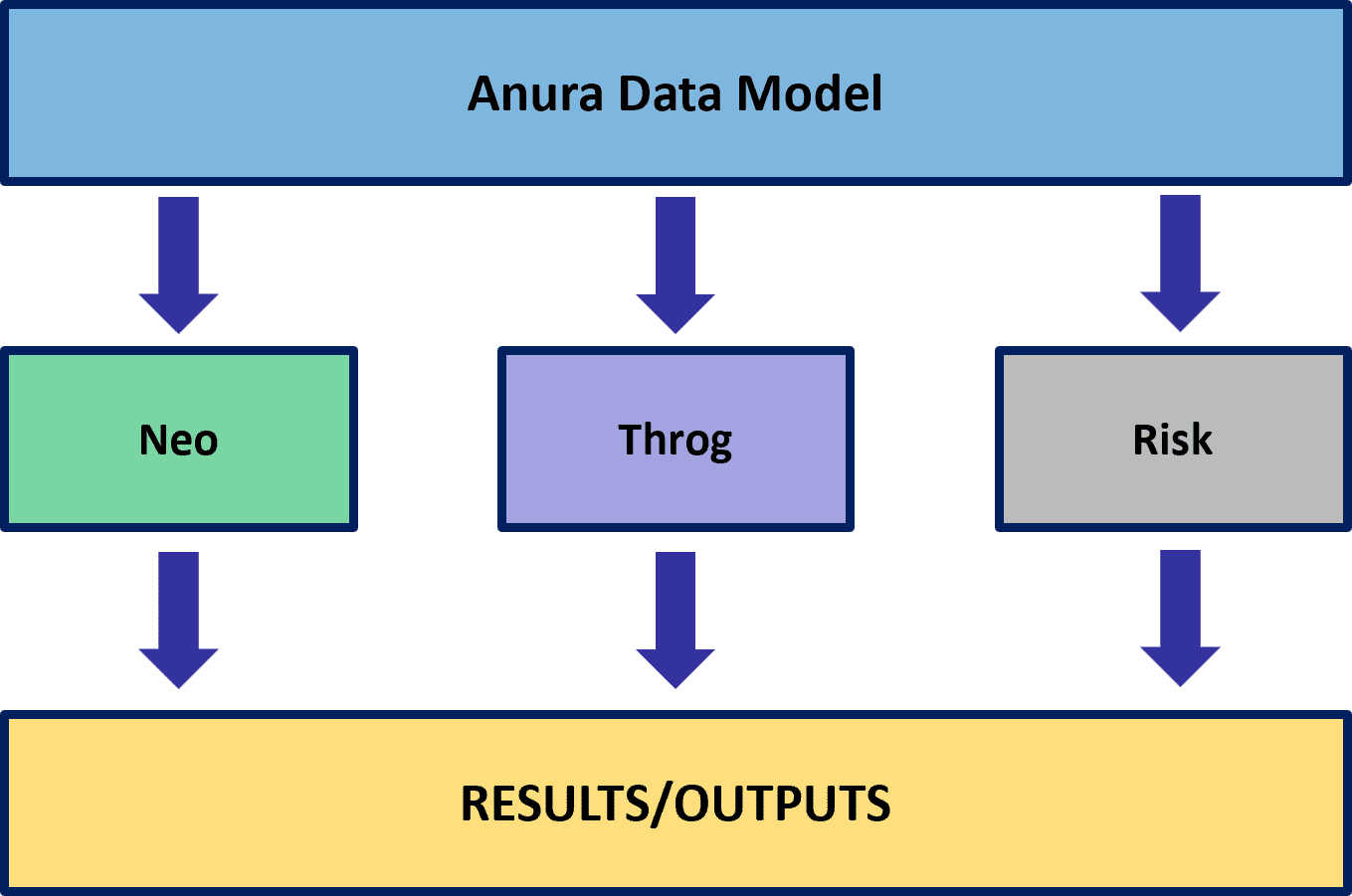
Anura is comprised of modeling categories required to build a model. Each modeling category contains tables to add pertinent detail and/or complexity to your model as well as identify structure, policies, costs, and constraints.
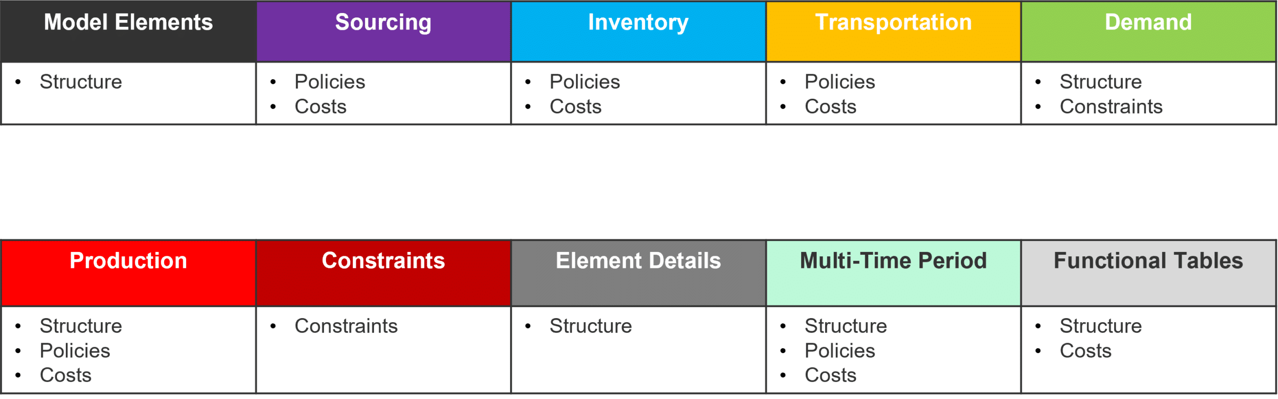
A complete list of the tables and fields within each table can be downloaded locally here.
The validation error report table will be populated for all model solves and contains a lot of helpful information for both reviewing and troubleshooting models. A set of results will be saved for each scenario and every record will report the table and column where the issue has been identified, a description of the error, the value that was identified as the problem along with the action taken by the solver. In the instance where multiple records are generated for the same type of error, you will see an example record populated as the identified value and a count of the errors will be displayed – detailed records can be printed using debug mode. Each record will also be rated on the severity of its impact on a scale from 0 – 3 with 3 being the highest.
The validation error report can serve as a great tool to help troubleshoot an infeasible model. The best approach for utilizing this table is to first sort on the Severity column so that the highest level issues are displayed. If severity 3 issues are present, they must be addressed. If no severity 3 issues exist, the next steps would be to review any severity 2 issues to consider policy impact. It is also helpful to search for any instances where rows are being dropped as these dropped rows will likely influence other errors. To do this, filter the Action field for ‘Row Dropped’.
While the report can be helpful in trying to proactively diagnose infeasible models, it won’t always have all of the answers. To learn more about the dedicated engine for infeasibility diagnosis please check out this article: Troubleshooting With The Infeasibility Diagnostic Engine
Severity 3 records capture instances of syntax issues that are preventing the model from being built properly. This can be presented as 2 types:
Severity 3 records can also be instances where model infeasibility can be detected before the model solve begins, in the instance where a severity 3 error is detected the model solve will be cancelled immediately. There are 3 common instances of these Severity 3 errors:
Severity 2 records capture sources of potential infeasibility and while not always a definitive reason for a problem being infeasible, they will highlight potential issues with the policy structure of a model. There are 2 common instances of Severity 2 errors:
These severity 2 errors don’t necessarily indicate a problem, they can often times be caused by grouped-based policies and members overlapping from one group to another. It is still a good idea to review these gaps in policies and make sure that all of the lanes which should be considered in your solve are in fact being read into the solver.
Severity 1 records will capture issues in model data that can cause rows from input tables to be dropped when writing the solver files for a model. These can be issues on allowed numerical ranges, a negative quantity for customer demand as an example. Detailed policy linkages that do not align can also cause errors, for example a process which uses a specific workcenter that doesn’t exist at the assigned facility. There are other causes of severity 1 errors, and it is important to review these errors for any changes that are made to your input data. Be sure to check the Action column to see if a default value was applied and note the new value that was used, or if a row was being dropped.
Severity 1 records will also note other issues that have been identified in the model input data. These can be unused model elements such as a customer which is included but has no demand, or transportation modes that exist in the model but aren’t assigned to any lanes. There can also be records generated for policies that have no cost charged against them to let you know that a cost is missing. Duplicate data records will also be flagged as severity 1 errors – the last row read in by the solver will be persisted. If you have duplicated data with different detailed information these duplicates should be addressed in your input tables so that you can make sure the correct information is read in by the solver.
A point to look out for is any severity 1 issue that is related to an invalid UOM entry – these will cause records to be dropped and while the dropped records don’t always directly cause model infeasibilities themselves, they can often times be at the root of other issues identified as higher severity or through infeasibility diagnosis runs.
Severity 0 records are for informational purposes only and are generated when records have been excluded upstream, either in the input tables directly or by other corrective actions that the solver has taken. These records are letting you know that the solver read in the input records but they did not correspond to anything that was in the current solve. An example of this would be if you only included a subset of your facilities for a scenario, but still had included records for an out-of-scope MFG location. If the MFG is excluded in the facilities table but its production policies are still included, a record will be written to the table to let you know that these production policy rows were skipped.
Utilities enable powerful modelling capabilities for use cases like integration to other services or data sources, repeatable data transformation or anything that can be supported by Python! System Utilities are available as a core capability in Cosmic Frog for use cases like LTL rate lookups, TransitMatrix time & distance generation, and copying items like Maps and Dashboards from one model to another. More useful System Utilities will become available in Cosmic Frog over time. Some of these System Utilities are also available in the Resource Library where they can be downloaded from, and then customized and made available to modelers for specific projects or models. In this Help Article we will cover both how to use use System Utilities as well as how to customize and deploy Custom Utilities.
The “Using and Customizing Utilities” resource in the Resource Library includes a helpful 15-minute video on Cosmic Frog Model Utilities and users are encouraged to watch this.
In this Help Article, System Utilities will be covered first, before discussing the specifics of creating one’s own Utilities. Finally, how to use and share Custom Utilities will be explained as well.
Users can access utilities within Cosmic Frog by going to the Utilities section via the Module Menu drop-down:
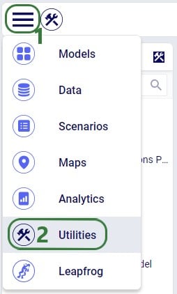
Once in the Utilities section, user will see the list of available utilities:
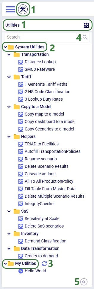
The appendix of this Help Article contains a table of all System Utilities and their descriptions.
Utilities vary in complexity by how many input parameters a user can configure and range from those where no parameters need to be set at all to those where many can be set. Following screenshot shows the Orders to Demand utility which does not require any input parameters to be set by the user:
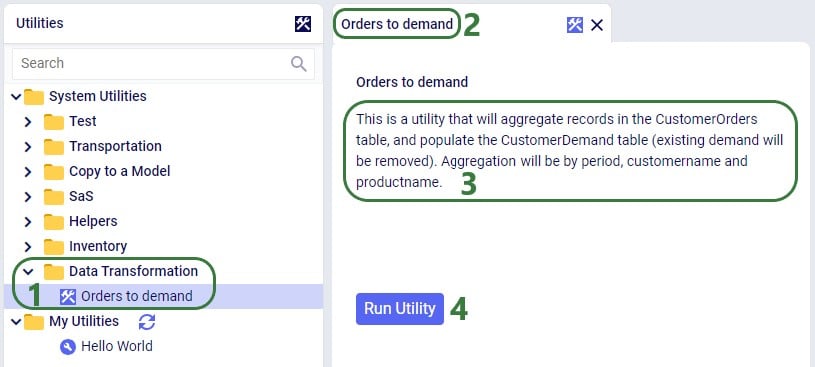
The Copy map to a model utility shown in the next screenshot does require several parameters to be set by the user:
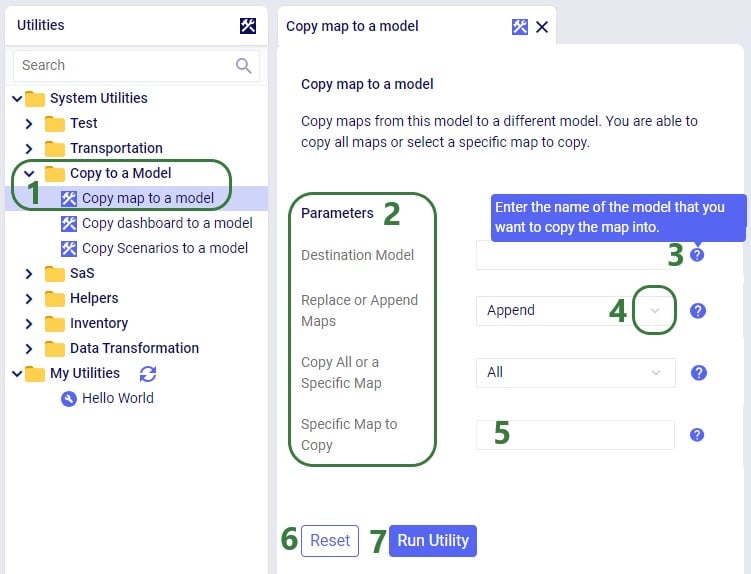
When the Run Utility button has been clicked, a message appears beneath it briefly:
Clicking on this message will open the Model Activity pane to the right of the tab(s) with open utilities:

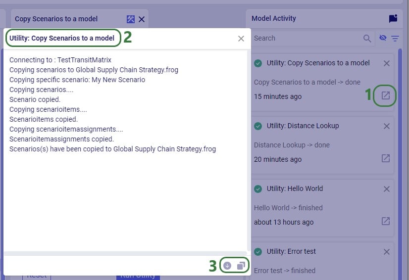
Users will not only see activities related to running utilities in the Model Activity list. Other actions that are executed within Cosmic Frog will be listed here too, like for example when user has geocoded locations by using the Geocode tool on the Customers / Facilities / Suppliers tables or when user makes a change in a master table and chooses to cascade these changes to other tables.
Please note that the following System Utilities have separate Help Articles where they are explained in more detail:
The utilities that are available in the Resource Library can be downloaded by users and then customized to fit the user’s specific needs. Examples are to change the logic of a data transformation, apply similar logic but to a different table, etc. Or users may even build their own utilities entirely. If a user updates a utility or creates a new one, they can share these back with other users so they can benefit from them as well.
Utilities are Python scripts that contain a specific structure which will be explained in this section. They can be edited directly in the Atlas application on the Optilogic platform or users can download the Python file that is being used as a starting point and edit it using an IDE (Integrated Development Environment) installed on their computer. A rich text editor geared towards coding, like for example Visual Studio Code, will work fine too for most. An advantage of working locally is that user can take advantage of code completion features (auto-completion while typing, showing what arguments functions need, catch incorrect syntax/names, etc.) by installing an extension package like for example IntelliSense (for Visual Studio Code). The screenshots of the Python files underlying the utilities that follow in this documentation are taken while working with them in Visual Studio Code locally and on a machine that has the IntelliSense extension package installed.
A great resource on how to write Python scripts for Cosmic Frog models is this “Scripting with Cosmic Frog” video. In this video, the cosmicfrog Python library, which adds specific functionality to the existing Python features to work with Cosmic Frog models, is covered in some detail.
We will start by looking at the Python file of the very simple Hello World utility. In this first screenshot, the parts that can stay the same for all utilities are outlined in green:

Next, onto the parts of the utility’s Python script that users will want to update when customizing / creating their own scripts:
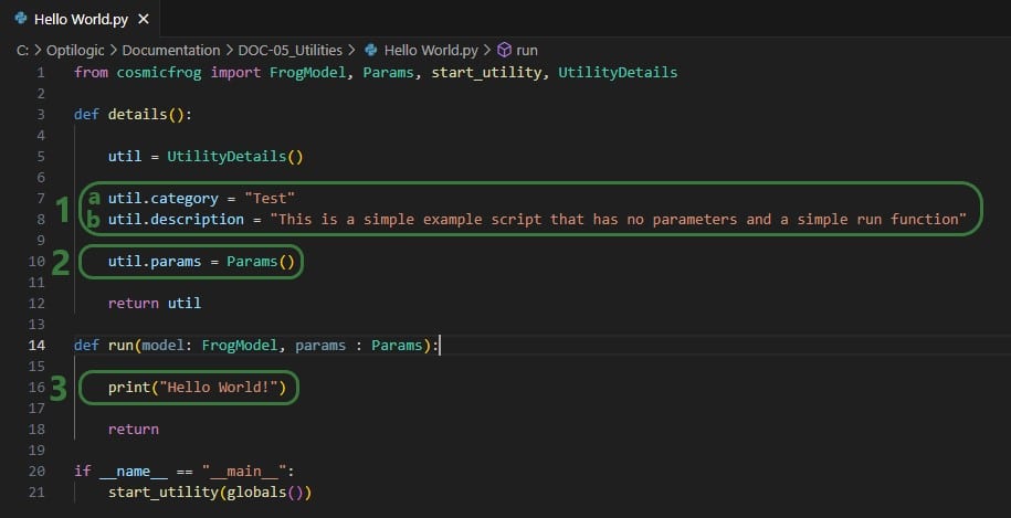
Now, we will discuss how input parameters, which users can then set in Cosmic Frog, can be added to the details function. After that we will cover different actions that can be added to the run function.
If a utility needs to be able to take any inputs from a user before running it, these are created by adding parameters in the details function of the utility’s Python script:

We will take a closer look at a utility that uses parameters and map the arguments of the parameters back to what the user sees when the utility is open in Cosmic Frog, see the next 2 screenshots: the numbers in the script screenshot are matched to those in the Cosmic Frog screenshot to indicate what code leads to what part of the utility when looking at it in Cosmic Frog. These screenshots use the Copy dashboard to a model utility of which the Python script (Copy dashboard to a model.py) was downloaded from the Resource Library.
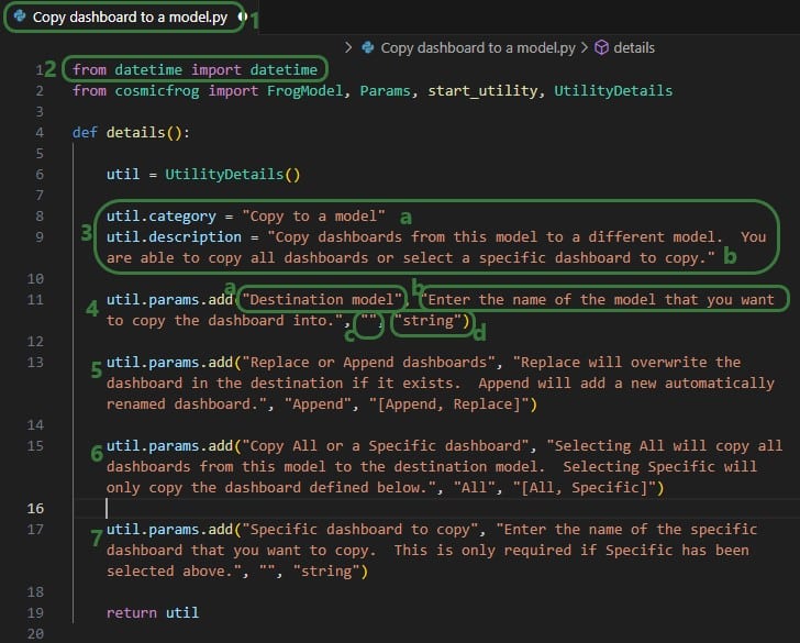
Note that Python lists are 0-indexed, meaning that the first parameter (Destination Model in this example) is referenced by typing params[0], the second parameter (Replace of Append dashboards) by typing params[1], etc. We will see this in the code when adding actions to the run function below too.
Now let’s have a look at how the above code translates to what a user sees in the Cosmic Frog user interface for the Copy dashboard to a model System Utility (note that the numbers in this screenshot match with those in the above screenshot):
The actions a utility needs to perform are added to the run function of the Python script. These will be different for different types of utilities. We will cover the actions the Copy dashboard to a model utility uses at a high level and refer to Python documentation if user is interested in understanding all the details. There are a lot of helpful resources and communities online where users can learn everything there is to know about using & writing Python code. A great place to start is on the Python for Beginners page on python.org. This page also mentions how more experienced coders can get started with Python. Also note that text in green font that follows a hash sign are comments to add context to code.
For a custom utility to be showing in the My Utilities category of the utilities list in Cosmic Frog, it needs to be saved under My Files > My Utilities in the user’s Optilogic account:
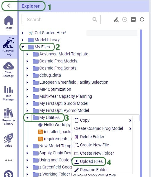
Note that if a Python utility file is already in user’s Optilogic account, but in a different folder, user can click on it and drag it to the My Utilities folder.
For utilities to work, a requirements.txt file which only contains the text cosmicfrog needs to be placed in the same My Files > My Utilities folder (if not there already):

A customized version of the Copy dashboard to a model utility was uploaded here, and a requirements.txt file is present in the same folder too.
Once a Python utility file is uploaded to My Files > My Utilities, it can be accessed from within Cosmic Frog:
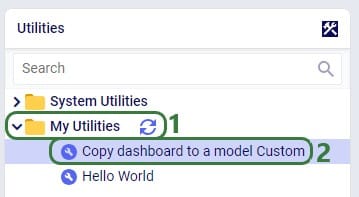
If users want to share custom utilities with other users, they can do so by right-clicking on it and choosing the “Send Copy of File” option:

The following form then opens:
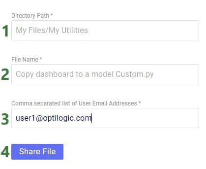
When a custom utility has been shared with you by another user, it will be saved under the Sent To Me folder in your Optilogic account:
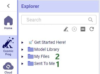
Should you have created a custom utility that you feel a lot of other users can benefit from and you are allowed to share outside of your organization, then we encourage you to submit it into Optilogic’s Resource Library. Click on the Contribute button at the left top of the Resource Library and then follow the steps as outlined in the “How can I add Python Modules to the Resource Library?” section towards the end of the “How to use the Resource Library” help article.
Utility names and descriptions by category:
Sequential Objectives allow for you to set multiple tiers of objectives for the optimization solve to consider, where each tier of objectives can be relaxed by a defined percentage when solving for the next tier.
Here is a basic example of how Sequential Objectives can be used.
100 units of demand for P1 at CZ.
Available pathways for flow are as follows:
Find a solution that will first minimize total costs, but then will work to minimize the total amount of travel time in the solution while only relaxing the Total Cost solution by 20%.
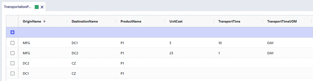
When just solving with the standard objective of Profit Maximization, the cheapest path will be utilized. All flows will come from MFG > DC1 > CZ and the total cost will be $500.
We’ve built the Sequential Objectives so that we will first optimize over the Total Supply Chain Cost as Priority 1. We have also set the Tolerance to be 20 which will allow for a 20% relaxation in the solution to solve for the secondary objective – Total Weighted Flow Time.
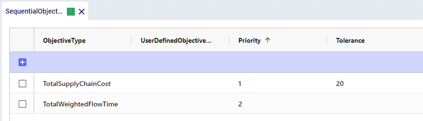
We’ll now see that the more expensive pathway of MFG > DC2 > CZ is used as it requires less travel time. Because the initial cost was $500, we will send as many units as possible through DC2 up until the total cost reaches $600 – a 20% deviation from the initial cost. This results is 5 units flowing via DC2, while 95 units remain through DC1 for a total cost of $600.
This example model can be found in the Resource Library listed under the name of Sequential Objectives Demo.
Running a model in debug mode can be a helpful troubleshooting tool as it will print more detailed reports of model issues.
The run option for Debug Mode is not included as a default in models but it can be added via the SQL Editor. Please copy and paste the following SQL query and run it against the model database you wish to add the option to.
Copy SQL Query Here: Add Debug Mode Model Run Option SQL Statement
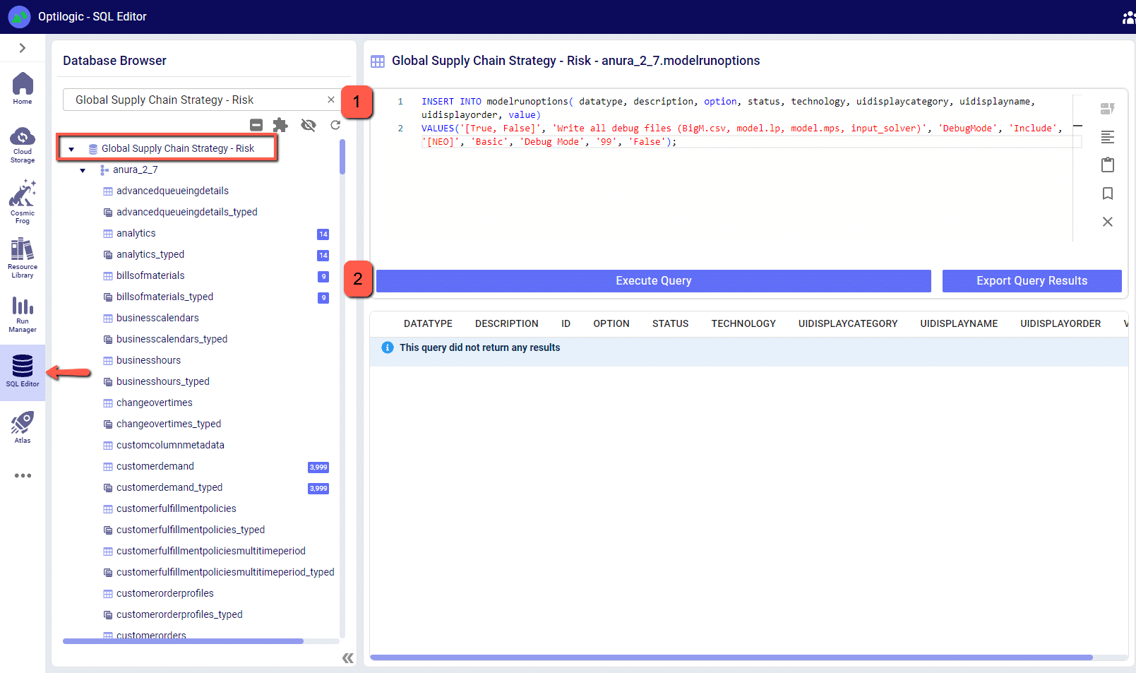
Now, if you open the model again in Cosmic Frog you will see that Debug Mode is an available option in the run screen.
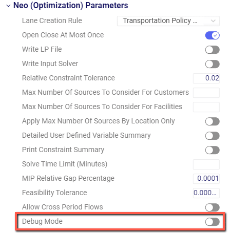
When set to True, Debug Mode will show all instances of validation errors instead of displaying an example of an error and the count of occurrences. You can see the difference in the following screenshot, where 1 row with 61 instances of the same error is turned into 61 individual rows.
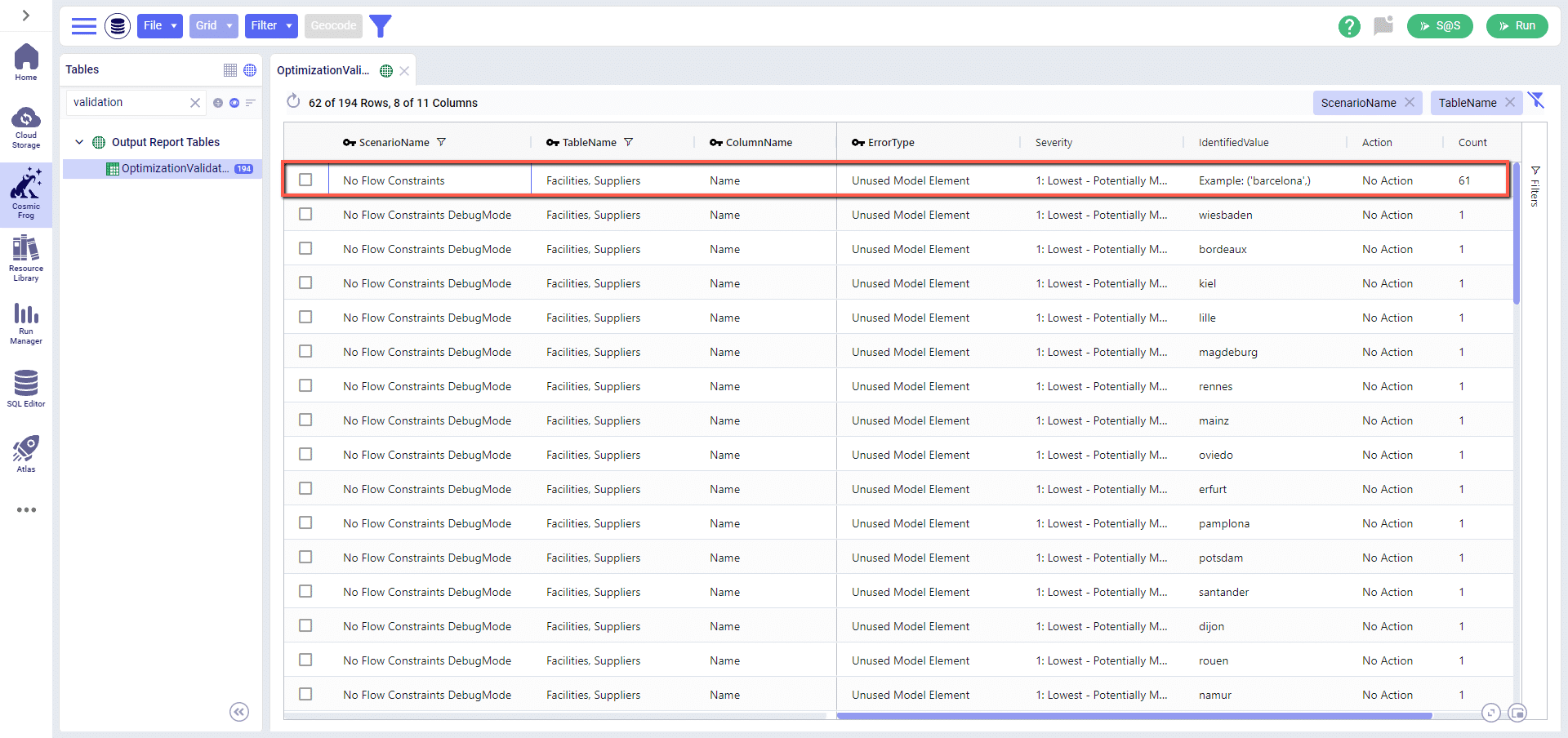
Debug Mode will also print and save the input files that are passed to the solver – these will be saved in your File Explorer at My Files > debug_data > ModelName > ScenarioName. For each scenario run with debug mode enabled you will have the following:
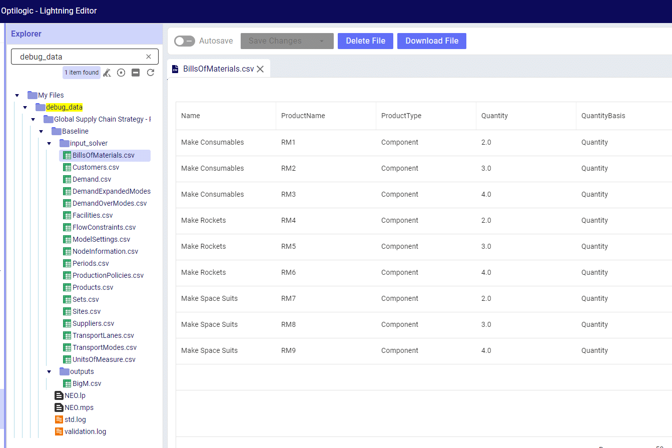
Please note that this data is saved to your File Explorer and for larger models can take up quite a bit of disk space. If you reach 100% disk space utilization you will be unable to run any new jobs as they won’t have any space to write their required data to. The debug_data folder is almost always the cause of this disk space utilization issue, clearing its contents will allow jobs to start again.
If you have any questions or concerns about how this might impact your models, please don’t hesitate to reach out to support@optilogic.com.
The nature of LTL freight rating is complex and multi-faceted. The RateWare® XL LTL rating engine of SMC3 enables customers to manage parcel pricing and LTL rating complexity, for both class and density rates, with comprehensive rating solutions.
Cosmic Frog users that hold a license to the RateWare XL LTL Rating Engine of SMC3 can easily use it within Cosmic Frog to lookup LTL rates and use them in their models. In this documentation we will explain where to find the SMC3 RateWare utility within Cosmic Frog and how to use it. First, we will cover the basic inputs needed in Cosmic Frog models, then how to configure and run the SMC3 RateWare Utility to look up LTL rates, and finally how to add those rates for usage in the model.
Before running the SMC3 RateWare Utility to retrieve LTL rates, we need to set up our model, including the origin-destination pairs for which we want to look up the LTL rates. Here, we will cover the inputs of a basic demo model showing how to use the SMC3 RateWare Utility. Of course, models using this utility may be much more complex in setup as compared to what is shown here.
The next 3 screenshots show:
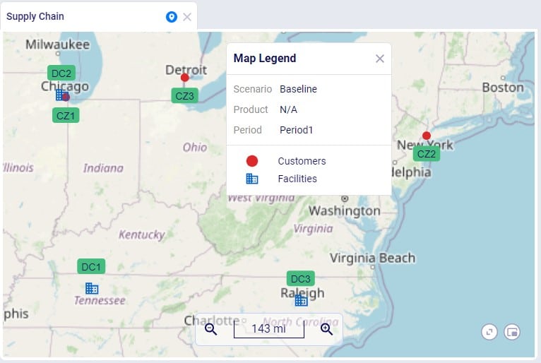
To facilitate model building, this model uses groups for Customer and DCs, as shown in the next screenshot. All DCs are members of the DCs group and all CZs are members of the Customers group:
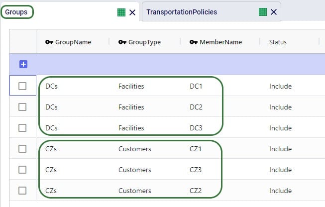
Using these groups, the Transportation Policies table is easily set up with 1 record from the DCs group to the CZs group as shown in the next screenshot. At runtime this 1 record is expanded into all possible OriginName-DestinationName combinations of the group members. So, this is an all DCs to all Customers policy that covers 9 possible origin-destination combinations.
Besides these tables, this simple model also has several other tables that are populated:
The SMC3 RateWare Utility is available by default from the Utilities module in Cosmic Frog, see next screenshot. Click on the Module Menu icon with 3 horizontal bars at the top left in Cosmic Frog, then click on Utilities in the menu that pops up:
You will now see a list of Utilities, similar to the one shown in this next screenshot (your Utilities are likely all expanded, whereas most are collapsed in this screenshot):
The rest of the inputs that can be configured are specific to the RateWare XL LTL Rating Engine and we refer user to SMC3’s documentation for the configuration of these settings.
When the utility is finished running, we can have a look at the smc3_inputs and smc3_outputs tables (if the option of All was used for Select Operation). First, here is a screenshot of the smc3_inputs table:

The next screenshot shows the smc3_outputs table in Optilogic’s SQL Editor. This is also a table with many columns as it contains origin and destination information, repeats the inputs of the utility, and contains details of the retrieved rates. Here, we are only showing the 3 most relevant columns: originname (the source DC), destinationname (the customer), and detailrate_1 which is the retrieved LTL rate:
Now that we have used the SMC3 RateWare Utility to retrieve the LTL rates for our 9 origin-destination pairs, we need to configure the model to use them as they are currently only listed in the smc3_outputs custom table. We use the Lookups table (an Input table in the Functional Tables section) to create a lookup link between the smc3_outputs custom table and the Transportation Policies input table, as follows:
To finalize setting up the Lookup, we now apply it to the UnitCost field on the TransportationPolicies table, where we set the field to the name of the Lookup, see screenshot below. Now, when the model is run, the 1 transportation policy is expanded into the 9 origin-destination pairs it represents and the Unit Cost field is populated with the detailrate_1 value of the smc3_outputs table based on matching origin name, destination name, and product name between the 2 tables.

Lastly, we run a network optimization (NEO engine) on our small example model and look at the Optimization Flow Summary output table:
The optimization has correctly used DC2 as the source for CZ1 as it has the lowest rate for going to CZ1 of the 3 DCs (see screenshot further above of the smc3_outputs table). The rate is 23.18 and for 10 units moved (FlowQuantity) this results in a TransportationCost of 231.80. Similarly, we can double-check that indeed DC2 has the cheapest rate for going to CZ3 as well, DC3 has the cheapest rate for going to CZ2, and the Transportation Costs are correctly calculated as the LTL rate * flow quantity.
The Resource Library is the application within the Optilogic platform where you can find files that will help facilitate, accelerate, and customize your model building and running. These include Cosmic Frog template models, Python scripts, Reference Data and more.
There are several ways to search, sort and filter the list of resources:

When a file in the list is selected by clicking on it, a Preview is shown on the right-hand side of the screen. This preview contains a short description of the resource, may contain a Video Introduction explaining for example the business problem or Cosmic Frog features covered in the resource, lists any Related (= included) Files, and lists any Tags that are associated with the resource so users can quickly understand what materials are covered by this resource.
You may want to add a new resource to the Resource Library if you think other users may be interested in the contents, for example to showcase a certain business problem modelled in Cosmic Frog, or to add Reference Data that can be helpful for others too, or to share the automation of a common model building/analysis step. On other occasions you may want to replace a resource in the library with an updated version. If you want to add or replace a resource in the library, you can do so by clicking on the Contribute button (found in the top-left corner of the Resource Library), and then follow the steps as explained in the next sections.
After clicking the Contribute button the following submission form will be shown:
The steps to contribute a Python Module to the Resource Library are very similar to those described above for adding a Cosmic Frog database:
If you find that the standard constraints or costs in a model don’t quite capture your specific needs, you can create and define your own variables to use with costs and constraints.
To help in framing this discussion, let’s start with a simple example that fits into the standard input tables.
We wouldn’t need to do anything special in this instance, just create policies as normal and attach a Unit Cost of 5 to the MFG > DC transportation policy. To apply the constraint, we would create a Flow Constraint that sets a Max flow of 1000 units. While the input requirements are straightforward in this instance, let’s define both objectives in terms of variables as the solver would see them.
Flow Variable: MFG_CZ_Product_1_Flow
This example is simple, but it is important to think about costs and constraints in terms of the variables that they are applied over. This becomes even more important when we want to craft our own variables.
Let’s modify the constraint in the example above to now restrict the flow of Product_1 between MFG and DC to be no more than the flow of Product_2. Again, we will represent this in terms of variables as the solver will see them.
Flow Variables: MFG_CZ_Product_1_Flow, MFG_CZ_Product_2_Flow
We no longer have a constant on the right-hand side of our constraint – this is an issue as we have no way to input this type of a constraint requirement into the Flow Constraints table. Whenever we find ourselves expressing constraints or costs in terms of other variables that will be determined based on the model solve, we will need to make use of User Defined Variables.
Continuing with the constraint above, let’s modify the inequality statement so that we do in fact have a constant on the right-hand side. We can do this by subtracting one of the variables from both sides of the statement – this will then leave the right-hand side as 0.
We now have a constraint that can be modelled but we need to be able to define the left-hand side through the User Defined Variables table. User Defined Variables are defined as a series of Terms which are all linked to the same Variable Name. Each Term can be thought of as a solver variable as we have defined them in the examples above. For each Term, we will also need to enter a Coefficient, the Type of behavior we want to be capturing, and all of the needed information in the columns that follow depending on the Type that was just selected. All of these columns are based off of the individual constraint tables, so it is helpful to think about data as if you were entering a row in the specific constraint table.
Here is how the inputs for our example would look set up as a User Defined Variable:
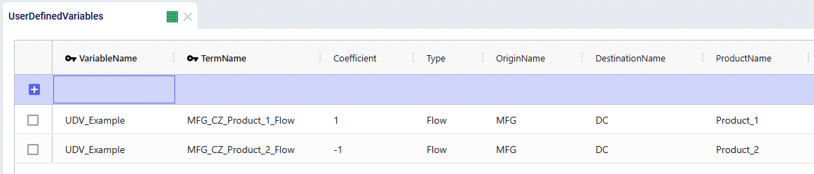
We can see that by using the coefficients of 1 and -1, we have now accurately built the left-hand side of our inequality statement. All that’s left is to link this to a User Defined Constraint.
User Defined Constraints can be used to add restrictions to the values captured by the User Defined Variables. All that is needed is to enter the corresponding Variable Name and then select the appropriate constraint type and value.
Revisiting our inequality statement once more, we can see how the User Defined Constraint should be built:
MFG_CZ_Product_1_Flow – MFG_CZ_Product_2_Flow <= 0
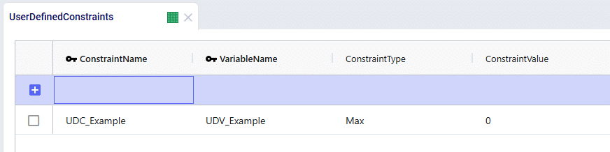
Watch the video to learn how to import, export, geocode, and work with data within Cosmic Frog:
If you want to follow along, please download the data set available here:
The Multi Time Period (MTP) tables allow for you to enter time-period specific data across many input tables. These MTP tables will act as overrides in the relevant periods for the records in their standard tables. If a record with the same key structure does not exist in the standard table, the MTP record won’t be recognized by the solver and will be dropped.
For example, we have a manufacturing facility with a throughput capacity of 1000 units. When this information is entered into the Facilities table, the throughput capacity will be used for each period in the model:
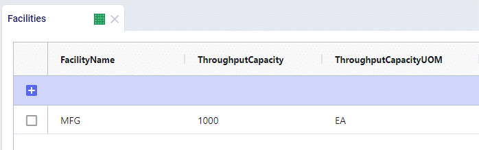
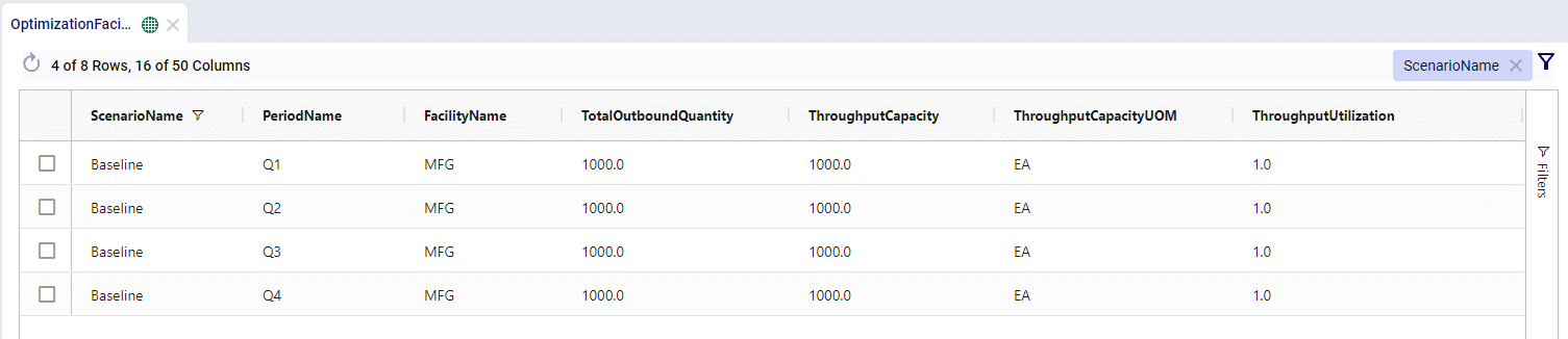
Let’s say that the manufacturing facility is expanding operations over the year and wants to show that the throughput capacity gradually increases over each quarter. This adjustment in throughput capacity can be defined in the Facilities Multi Time Period table:

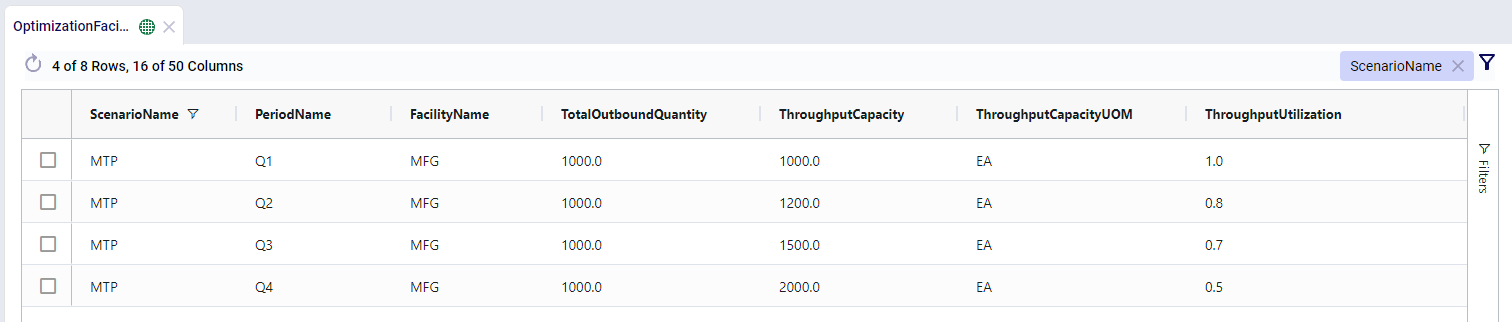
We can see that the throughput capacity increased over time and given the constant outbound quantity, the throughput utilization goes down as the model progresses.
In all of the policy multi-time period tables, there are two fields which appear to be similar – Status and Policy Status.
For example, we have 2 manufacturing locations that can produce the same product at very different costs. We’ll see that the MFG location is used as the sole production option as it is far cheaper.
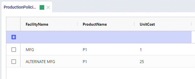
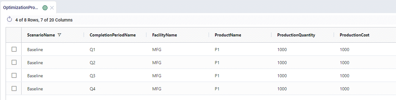
Now let’s say that we have to shut production down at the MFG location for maintenance in Q3, we can do this through the Production Policies Multi Time Period table:
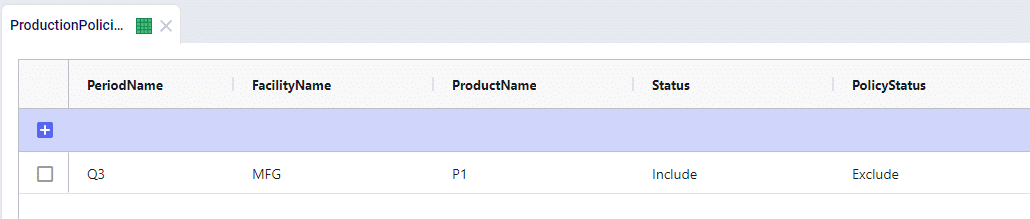
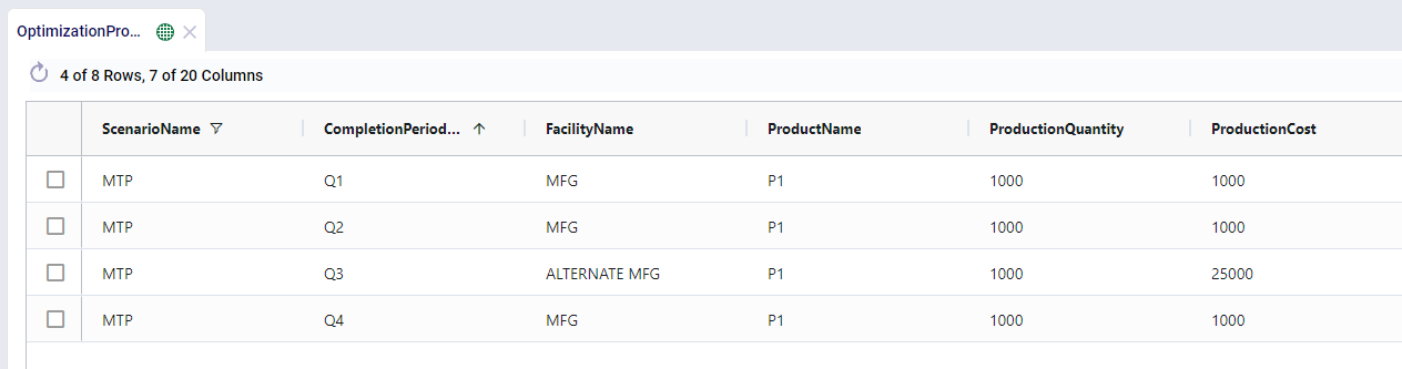
This can be a quick way to to adjust policies over different times and is an alternative to using constraints. The use of Policy Status in place of constraints will stop the creation of extra solver variables as well as reducing the number of constraints being placed over the solution. This can help contribute to better model performance.
Similar to how Status and Policy Status work, you have the ability to change the operating status of a Facility and a Work Center over time. This would allow you to Open, Close, or Consider the use of a Facility or Work Center in any given period.
Using the same example as above, we can model the maintenance at MFG during Q3 by closing the entire location:
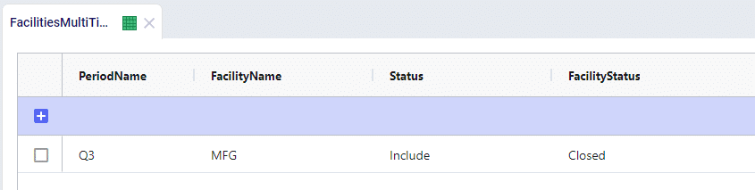
Closing the entire facility will do more than just limit production, the facility is then completely removed from the network for that given period and no other activities can take place.
Watch the video to learn how to connect your data tool of choice directly to your Optilogic model:
An example of how to connect a Cosmic Frog model to a Snowflake database, along with a video walkthrough, can be found in the Resource Library. To get a copy of this demo into your own Optilogic account simply navigate to the Resource Library and copy the Snowflake template into your workspace.
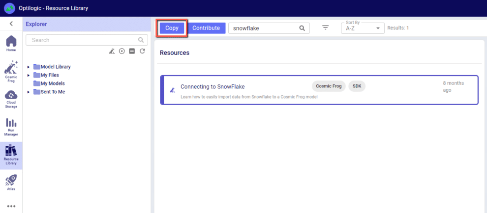
The following instructions show how to establish a local connection, using Alteryx, to an Optilogic model that resides within our platform. These instructions will show you how to:
Watch the video for an overview of the connection process:
A step by step set of instructions can also be downloaded in the slide deck here: CosmicFrog-Alteryx-Connection-Instructions
To make a local connection you must first open a Firewall connection between your current IP address and the Optilogic platform. Navigate to the Cloud Storage app – note that the app selection found on the left-hand side of the screen might need to be expanded. Check to see if your current IP address is authorized and if not, add a rule to authorize this IP address. You can optionally set an expiration date for this authorization.

If you are working from a new IP Address, a banner notification should be displayed to let you know that the new IP Address will need to be authorized.
From the Databases section of the Cloud Storage page, click on the database that you want to connect to. Then, click on the Connection Strings button to display all of the required connection information.
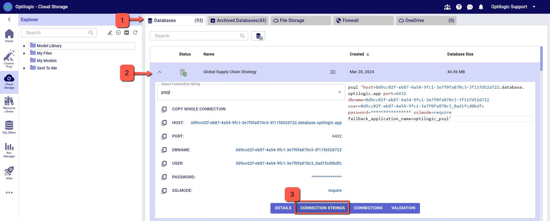
We have connection information for the following formats:
To select the format of your connection information, use the drop-down menu labeled Select Connection String:
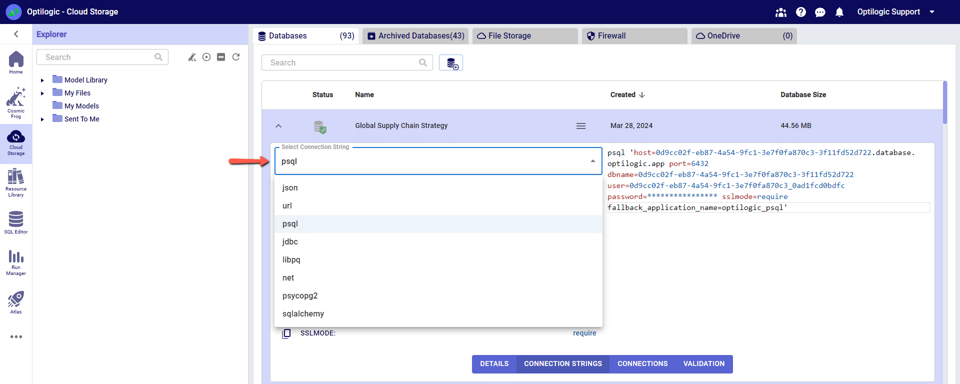
For this example, we will copy and paste the strings for the ‘PSQL’ connection. The screen should look something like the following:
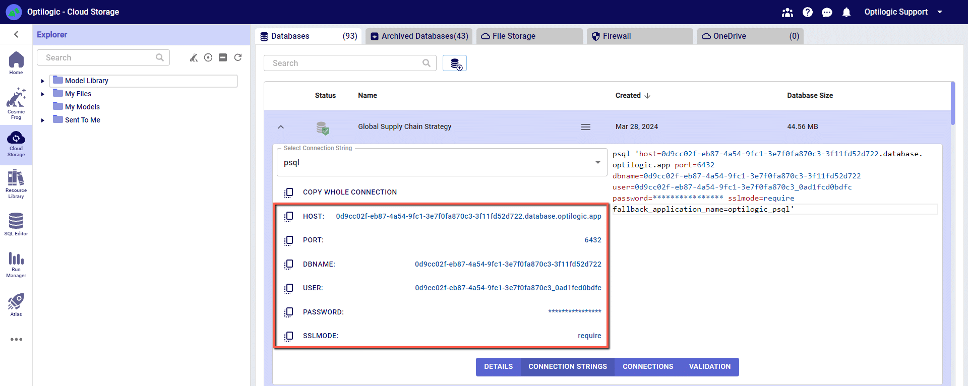
You can click on any of the parameters to copy them to your clipboard, and then paste them into the relevant field when establishing the PSQL ODBC connection.
Many tools, including Alteryx, use Open Database Connectivity (ODBC) to enable a connection to the Cosmic Frog model database. To access the Cosmic Frog model, you will need to download and install the relevant ODBC drivers. Latest versions of the drivers are located here: https://www.postgresql.org/ftp/odbc/releases/
From here, click on the latest parent folder, which as of June 20, 2024 will be REL-16_00_0005. Select and download the psqlodbc_x64.msi file.
When installing, use the default settings from the installation wizard.
At this point we have the pieces to make a connection in Alteryx. Open Alteryx and start a new Workflow. Drag the Input Data action into the Workflow and click to “Connect a File or Database.”
Select “Data sources” and scroll down to select “PostgresSQL ODBC”
On the next screen click “ODBC Admin” to setup the connection.
Click “Add” to create a new connection and then select “PostgreSQL ANSI(x64)” then click “Finish.”

Now we need to configure the connection with the information we gathered from the connection strings.
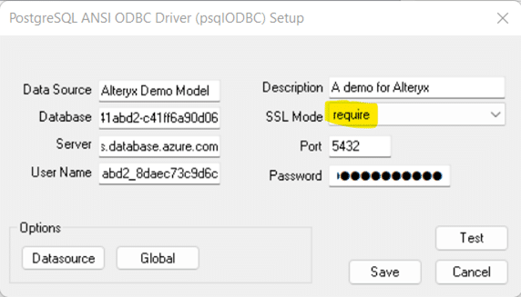
“Data Source” and “Description” allow you to name the connection, these can be named whatever you wish.
Copy the values for “Server”, “Database”, “User Name”, “Password” and “Port” from the connection string information copied from Optilogic Cloud Storage (see above).
DON’T FORGET to select “require” in “SSL Mode”
You may click “Test” to confirm the connection works or click “Save.”
Now select the new connection, in this example “Alteryx Demo Model” and click “OK”
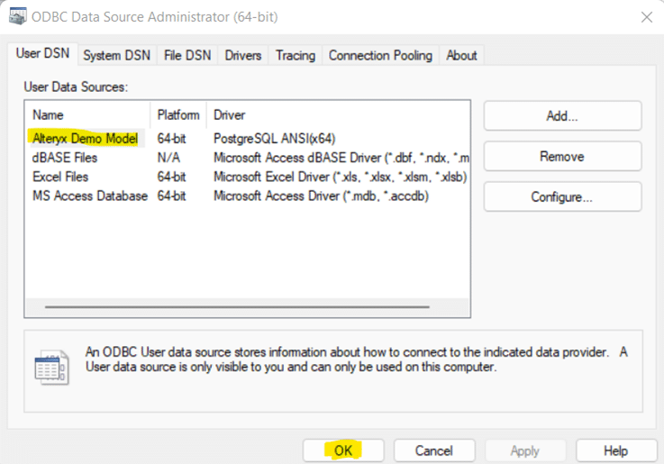
Now we need to select the same Data Source that we just built in ODBC within Alteryx. We need to enter the username and password for the connection for Alteryx authentication. These are the same credentials used to setup the ODBC connection. Remember to use your specific model’s credentials from the Connection String in the Optilogic platform Cloud Storage page.
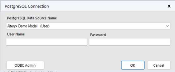
Depending on your organization’s security protocols, one additional step might need to be taken to whitelist Optilogic’s Postgres SQL Server. This can be done by whitelisting the host URL (*.postgres.database.azure.com) and the port (6432). If you are unsure how to whitelist the server or do not have the necessary permissions, please contact your IT department or network administrator for assistance.
11/16/2023 – There is an issue connecting through ODBC with the latest version of Alteryx. While we await a fix in an updated version of Alteryx, you can still connect with an older version of Alteryx (2021.4.2.47884)
05/01/2024 – Alteryx has resolved the ODBC connection issue with their latest major version release of 2024.1. If your currently installed Alteryx version is not working as intended, please upgrade to latest.
An alternative workaround is to disable the AMP engine on your Alteryx workflow. For any workflows that use the ODBC connection to a database hosted on the platform, you can uncheck the option in the Workflow Configuration for ‘Use AMP Engine’. The Workflow Configuration window will display on the left side of your screen if you click on the whitespace anywhere in your workflow.
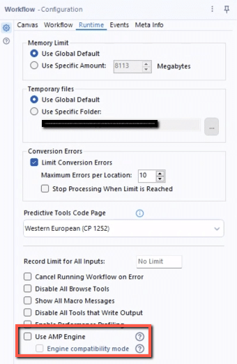
The following instructions show how to establish a local connection, using Azure Data Studio, to an Optiogic model that resides in the platform. These instructions will show you how to:
Watch the video for an overview of the connection process:
To make a local connection you must first open a Firewall connection between your current IP address and the Optilogic platform. Navigate to the Cloud Storage app – note that the app selection found on the left-hand side of the screen might need to be expanded. Check to see if your current IP address is authorized and if not, add a rule to authorize this IP address. You can optionally set an expiration date for this authorization.
If you are working from a new IP Address, a banner notification should be displayed to let you know that the new IP Address will need to be authorized.
From the Databases section of the Cloud Storage page, click on the database that you want to connect to. Then, click on the Connection Strings button to display all of the required connection information.
We have connection information for the following formats:
To select the format of your connection information, use the drop-down menu labeled Select Connection String:
For this example, we will copy and paste the strings for the ‘PSQL’ connection. The screen should look something like the following:
You can click on any of the parameters to copy them to your clipboard, and then paste them into the relevant field in Azure Data Studio when establishing the PSQL connection.
Within Azure Data Studio click the “Extensions” button and type in “postgres” in the search box to find and install the PostgreSQL extension.
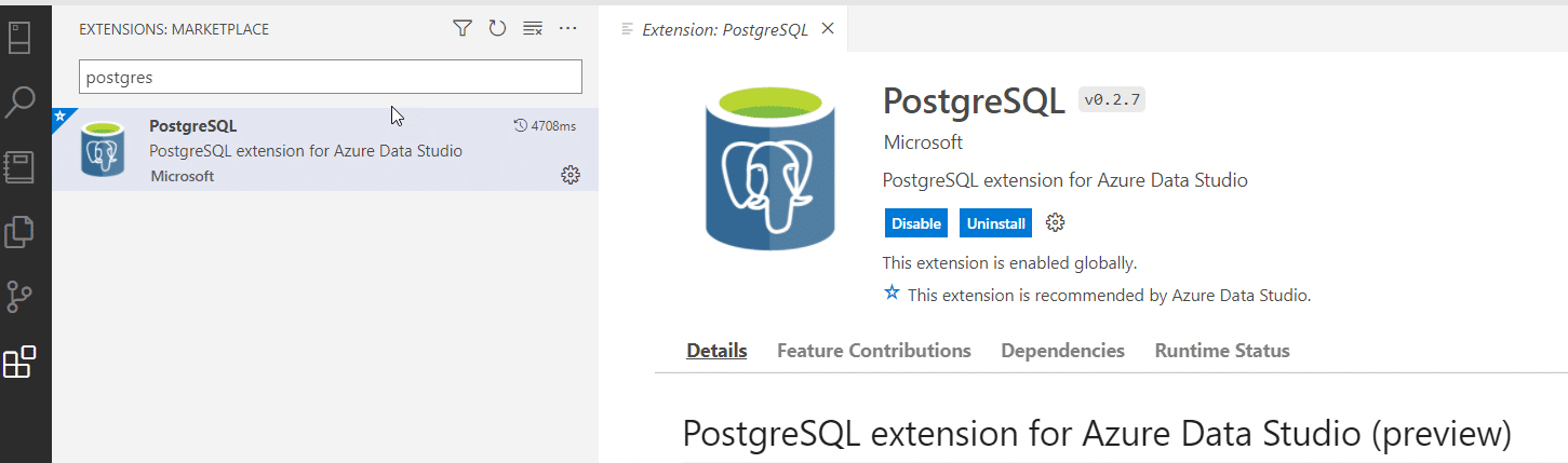
Add a new connection in Azure Data Studio, change the connection type to “PostgreSQL, “and enter the arguments for “PSQL” from the Cloud Storage page. NOTE: you will need to click “Advanced” to type in the Port and to change the SSL mode to “require.”
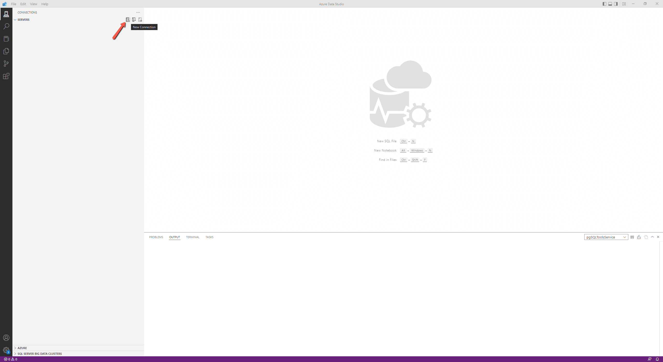
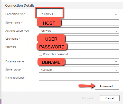
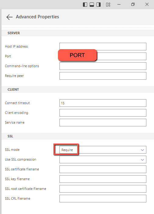
Depending on your organization’s security protocols, one additional step might need to be taken to whitelist Optilogic’s Postgres SQL Server. This can be done by whitelisting the host URL (*.database.optilogic.app) and the port (6432). If you are unsure how to whitelist the server or do not have the necessary permissions, please contact your IT department or network administrator for assistance.
The following instructions show how to establish a local connection, using Power BI, to an Optilogic model that resides within our platform. These instructions will show you how to:
To make a local connection you must first open a Firewall connection between your current IP address and the Optilogic platform. Navigate to the Cloud Storage app – note that the app selection found on the left-hand side of the screen might need to be expanded. Check to see if your current IP address is authorized and if not, add a rule to authorize this IP address. You can optionally set an expiration date for this authorization.
If you are working from a new IP Address, a banner notification should be displayed to let you know that the new IP Address will need to be authorized.
From the Databases section of the Cloud Storage page, click on the database that you want to connect to. Then, click on the Connection Strings button to display all of the required connection information.
We have connection information for the following formats:
To select the format of your connection information, use the drop-down menu labeled Select Connection String:
For this example, we will copy and paste the strings for the ‘PSQL’ connection. The screen should look something like the following:
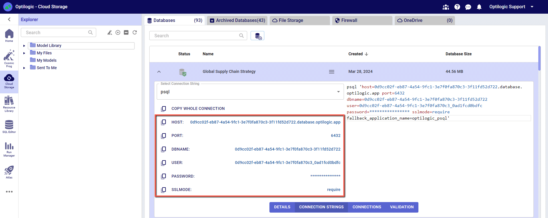
You can click on any of the parameters to copy them to your clipboard, and then paste them into the relevant field when establishing the PSQL ODBC connection.
Many tools, including Alteryx, use Open Database Connectivity (ODBC) to enable a connection to the Cosmic Frog model database. To access the Cosmic Frog model, you will need to download and install the relevant ODBC drivers. Latest versions of the drivers are located here: https://www.postgresql.org/ftp/odbc/releases/
From here, click on the latest parent folder, which as of June 20, 2024 will be REL-16_00_0005. Select and download the psqlodbc_x64.msi file.
When installing, use the default settings from the installation wizard.
Within Windows, open the ODBC Data Sources App (hint search: “ODBC” in your Windows spotlight search).
Click “Add” to create a new connection and then select “PostgreSQL ANSI(x64)” then click “Finish.”
Enter the details from your Cloud Storage connection — (hint: click to copy/paste)
You may click “Test” to confirm the connection works or click “Save.”
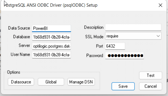
Open Power BI and select “Get data from another source”

Enter “ODBC” in the Get Data window and select connect
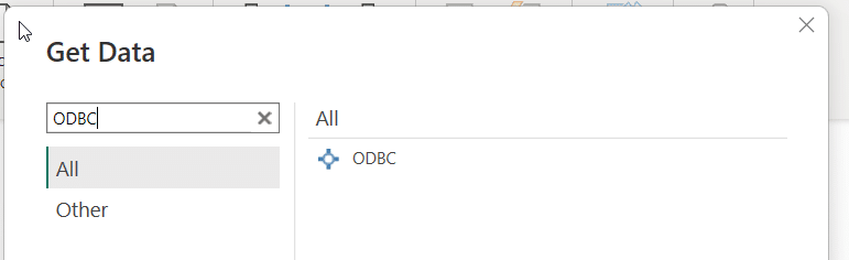
Select your Database connection from the dropdown and click OK
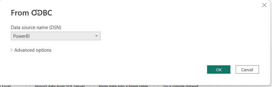
Enter your username and password one last time from the Cloud Storage page
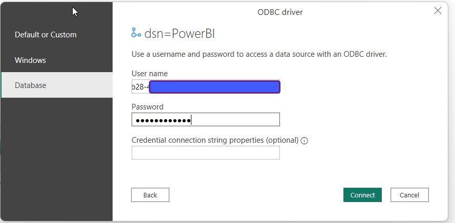
Select the tables you wish to see and use within PowerBI
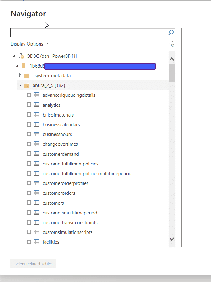
Create Dashboards of Data from Cosmic Frog tables!