We have prepared step-by-step instructions to build your own version of the Global Supply Chain Strategy model from scratch.
Please download the “Build your first Frog model.zip” file, save to your local machine, and follow the overview and instructions laid out in the following videos.
Python models can be run on your “local” IDE instance or you can leverage the power of hyper-scaling by running the module as a Job. When running as a job you have access to a number of different machine configurations as follows:
For reference, a typical laptop will be equivalent to either a XS or S machine configuration.
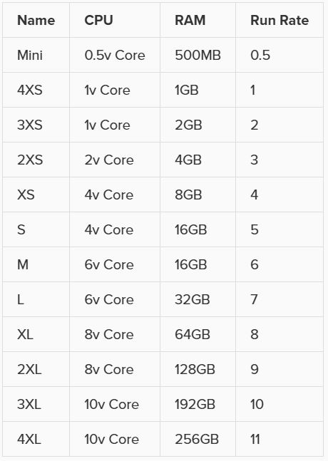
Complex optimization models may require more CPU cores to solve quickly and large scale simulations may require the use of more RAM due to increase in data required for model fidelity.
When modeling supply chains, stakeholders are often interested in understanding the cost to serve specific customers and/or products for segmentation and potential reposition purposes. In order to calculate the cost to serve, variable costs incurred all along the path through the supply chain need to be aggregated, while fixed costs that are incurred need to be apportioned to the correct customer/product. This is not always straightforward and easy to do, think for example of multi-layer BOMs.
When running a network optimization (using the Neo engine) in Cosmic Frog, these cost to serve calculations are automatically done, and the outputs are written into three output tables. In this help center article, we will cover these output tables and how the calculations underneath to populate them work.
First, we will briefly cover the example model used for screenshots for most of this help center article, then we will cover the 3 cost to serve output tables in some detail, and finally we will discuss a more complex example that uses detailed production elements too.
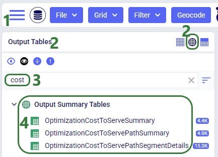
There are 3 network optimization output tables which contain cost to serve results; they can be found in the Output Summary Tables section of the output tables list:
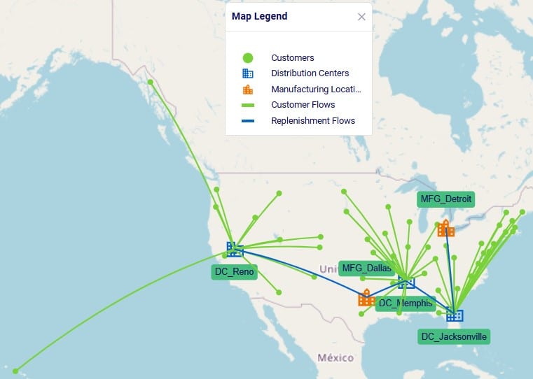
We will cover the contents and calculations used for these tables by using a relatively simple US Distribution model, which does use quite a few different cost types in it. This model consists of:
Following screenshot shows the locations and flows of one of the scenarios on a map:
One additional important input to mention is the Cost To Serve Unit Basis field on the Model Settings input table:

User can select Quantity, Volume, or Weight. This basis is used when needing to allocate costs based on amounts of product (e.g. amount produced or moved). For example, we need to allocate $100,000 fixed operating cost at DC_Raleigh to 3 outbound flows. The result is different when we use a different cost to serve unit basis:
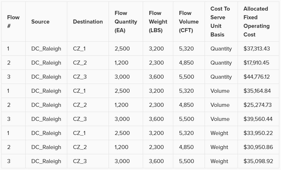
Note that in this documentation the Quantity cost to serve unit basis is used everywhere, which is the default.
We will cover the 3 output tables related to Cost To Serve using the above described model as an example in the screenshots. Further below in the document, we will also show an example of a model that uses some detailed production inputs and its cost to serve outputs. Let us start with examining the most detailed cost to serve output table, the Cost To Serve Path Segment Details table. This output table contains each segment of each path, from the most upstream product source location to customer fulfillment, which is the most downstream location. Each path segment represents an activity along the supply chain: this can be a production when product is made/supplied, inventory that is held, a flow where product is moved from one location to another, or use of a bill of materials when raw materials are used to create intermediates or finished goods.
Note that these output tables are very wide due to the number of columns they contain. In the screenshots, columns are often re-ordered, and some may be hidden if they do not contain any values or are not the topic of discussion, so they may not look exactly the same as what you see in your Cosmic Frog. Also, grids are often sorted to show records in increasing order of path ID and/or segment sequence.
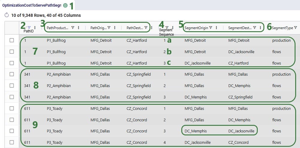
Please note that several columns are not shown in the above screenshot, these include:
Removing some additional columns and scrolling right, we see a few more columns for these same paths:
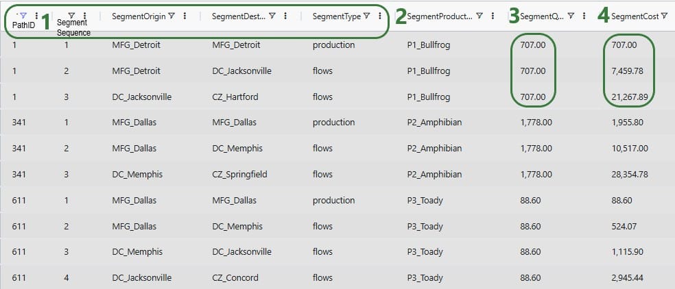
We will stay with the example of the path from MFG_Detroit to DC_Jacksonville to CZ_Hartford for 707 units of P1_Bullfrog to explain the costs (Path ID = 1 in the above). Here is a visual of this path, shown on the map:
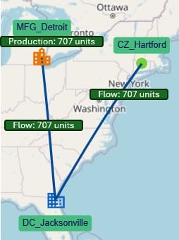
The following 4 screenshots show the 3 segments of this path in the Optimization Cost To Serve Path Segment Details output table, and the different costs that are applied to each segment. In this first screenshot, the left most column is the Segment Sequence, and a couple of fields that were not present in the screenshots above are now shown:



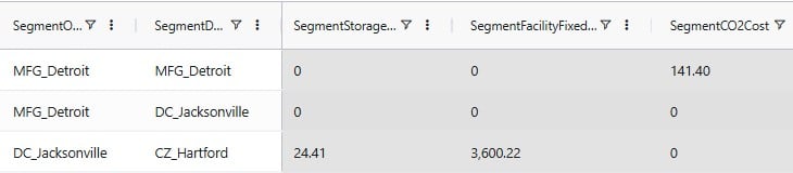
Let us put these on a map again, together with the calculations:

There are 2 types of costs associated with the production of 707 units of P1_Bullfrog at MFG_Detroit:
For the flow of 707 units from MFG_Detroit to DC_Jacksonville, there are 4 costs that apply:
There are 7 different costs that apply to the flow of the 707 units of P1_Bullfrog from DC_Jacksonville to CZ_Hartford where it fulfills the customer’s demand of 707 units:
There are cost fields in the Optimization Cost To Serve Path Segment Details output table that are not shown in the above screenshots as these are all blank in the example model used. These fields and their calculations should there be inputs to calculate them are as follows:
In the above examples we have seen Segment Types of production and flow. When inventory is modelled, we will also start seeing segments with Segment Type = inventories, as shown in this next screenshot (Cosmic Frog outputs of the Optimization Cost To Serve Path Segment Details table were copied into Excel from which the screenshot was then taken):
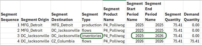
Here, 75.41 units of product P4_Polliwog were produced at MFG_Detroit in period 2025 (segment 1), then moved to DC_Jacksonville in the same period (segment 2), where they have been put into inventory (segment 3). These units are then used to fulfill customer demand at CZ_Columbia in the next period, 2026 (segment 4).
The Optimization Cost To Serve Path Segment Details table can also contain records which have Segment Type = no_activity. On these records there is no Segment Origin – Segment Destination pair, just one location which is not being used during the period (0 throughput). This record is then used to allocate fixed operating, startup, and/or closing costs to that location.
There are still a few fields in the Optimization Cost To Serve Path Segment Details table that have not been covered so far, these are:
The Optimization Cost To Serve Path Summary table is an output table which is an aggregation of the Optimization Cost To Serve Path Segment Details table, aggregated by Path ID. In other words, the table contains 1 record for each path where all costs of the individual segments of the path are rolled up into 1 number. Therefore, this table contains many of the same fields as the Path Segment Details table, just not the segment specific ones. The next screenshot shows the record for Path ID = 1 of the Optimization Cost To Serve Path Summary table:

This output table summarizes the cost to serve at the customer-product-period level and this table can be used to create reports at the customer or product level by aggregating further.
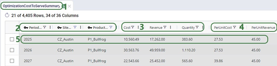
Note that all these 3 output tables can also be used in the Analytics module of Cosmic Frog to create any cost to serve dashboards. For example, this Optimization Cost To Serve Summary output table is used in 2 standard analytics dashboards that are part of any new Cosmic Frog model and will be automatically populated when this table is populated after a network optimization (Neo) run: the “CTS Unprofitable Demand” and “CTS Customer Profitability” dashboards. Here is a screenshot of the charts included in this second dashboard:
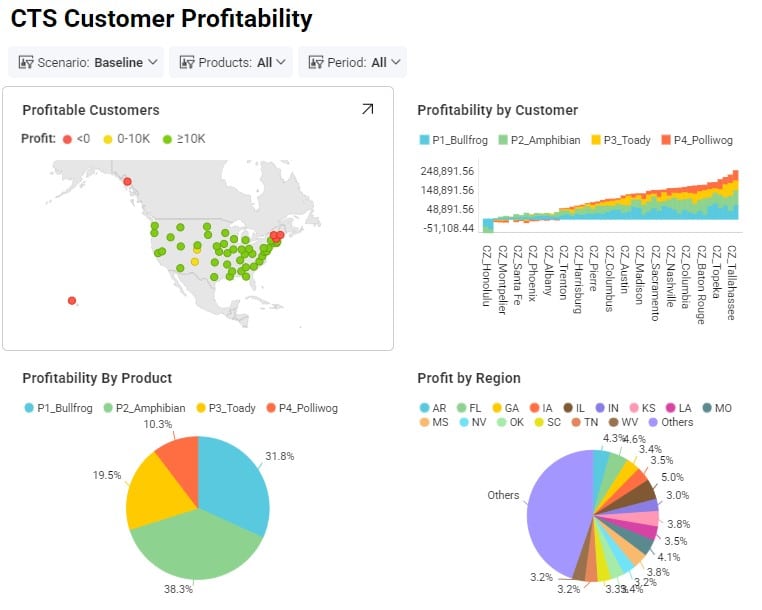
To learn more about the Analytics module in Cosmic Frog, please see the help center articles on this page.
In the above discussion of cost to serve outputs, the example model used did not contain any detailed production inputs, such as Bills Of Materials (BOMs), Work Centers, or Processes. We will now look at an example where these are used in the model and specifically focus on how to interpret the Optimization Cost To Serve Path Segment Details output table when bills of materials are included.
Consider the following records in the Bills of Materials input table for making the finished good FG_BLU (blue cheese):
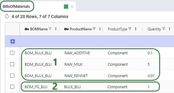
In the model, these BOMs are associated through Production Policies for the BULK_BLU and FG_BLU products.
Next, we will have a look at the Optimization Cost To Serve Path Segment Details output table to understand how costs are allocated to raw material vs finished good segments:
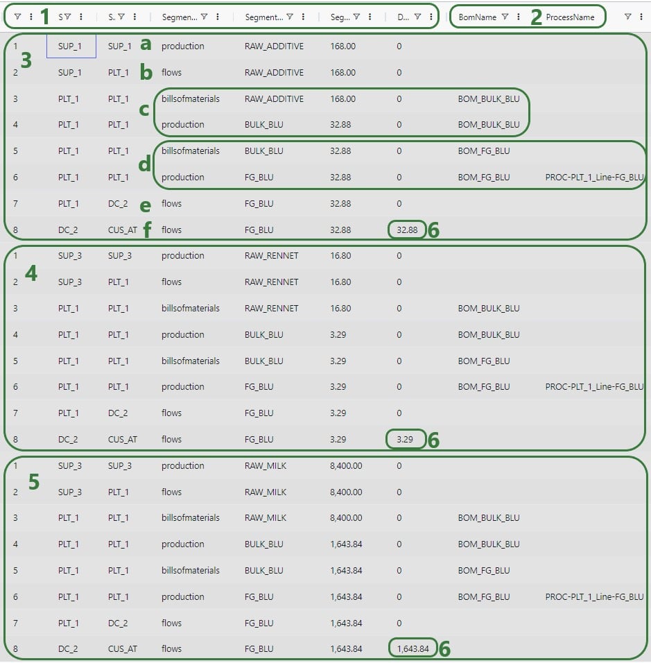
As we have seen before, there are many more cost columns in this table, so for each segment these can be reviewed by scrolling right. Finally, let’s look at these 3 paths in the Optimization Cost To Serve Path Summary output table:
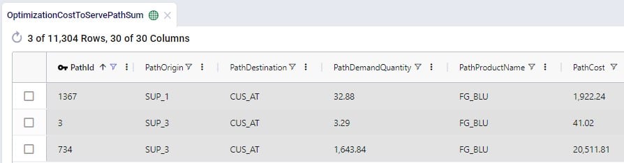
Note that the Path Product Name is FG_BLU for these 3 paths and there are no details to indicate which raw materials each of the paths pertains to. If required, this can be looked up using the Path IDs from this table in the Optimization Cost To Serve Path Segment Details output table.
Optilogic provides a uniform, easy to use way to connect to your models and embed optimization and simulation in any application that can make an API call.
With a free account you have access to our API capabilities to build and deploy custom solutions.
There are a number of calls that you will need to make to fully automate the use of optimization and simulation in your models. Below you will find more information on how to go about this task.
For full API documentation see our Optilogic API Documentation. From this page you will be able to view detailed API documentation and live test code within your account.
First, to use any API call you must be authenticated. One authenticated you will be provided with an API key that remains active for an hour. If your API key expires you will be required to re-authenticate to acquire a new key.
The Account API section of calls allows you to lookup your account information such as username, email, how many concurrent solves you have access to, and the number of workspaces in your account.
The Workspace API section of calls allows you to lookup information about a specific workspace. You can look up the workspace by name, obtaining a list of files in the workspace as well as a list of jobs associated with the models of that workspace.
The Job API section of calls allows you to view information relating to jobs in the system. Each time you execute a model solve, the Optilogic back end solver system, Andromeda, will spawn a new job to handle the request. The API call to start a job will return a key with which you can lookup information about that job, even after it has completed. With these API calls you can get any job’s status, start a new job, or delete a particular job.
The Files API section of calls allows you to interact with the files of a given workspace. Each model is made up of a collection of files (mainly code and data files). With these calls you can copy, delete, upload or download any file of in a specified workspace.
If this isn’t your first time using a supply chain design software, then take heart: the transition to Cosmic Frog is a smooth one. There are a few key differences worth noting below:
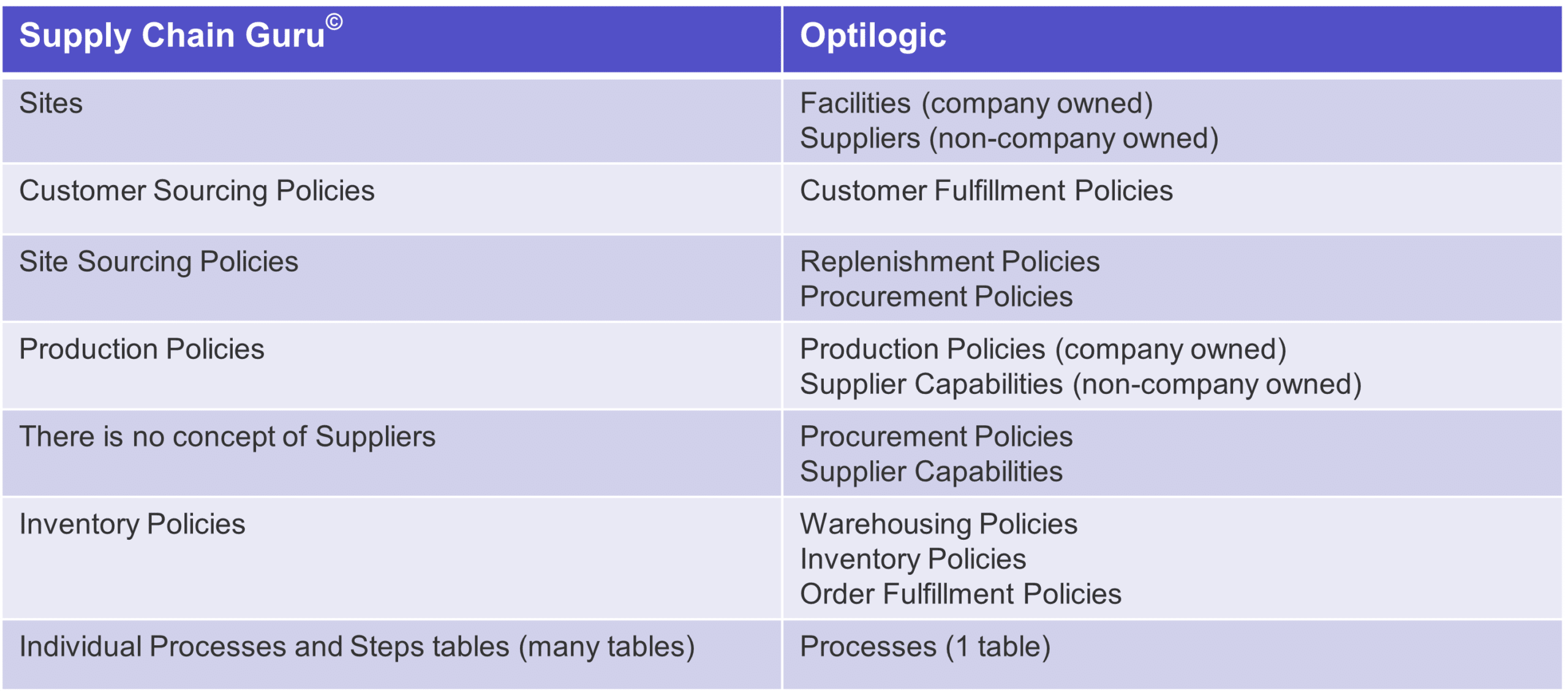
Most of these changes will be self-explanatory – if you used to write Customer Sourcing Policies you will now put similar data in a table called Customer Fulfillment Policies. Others may become easier to see over time — instead of many tables to create process logic you can enter everything you need in one table.
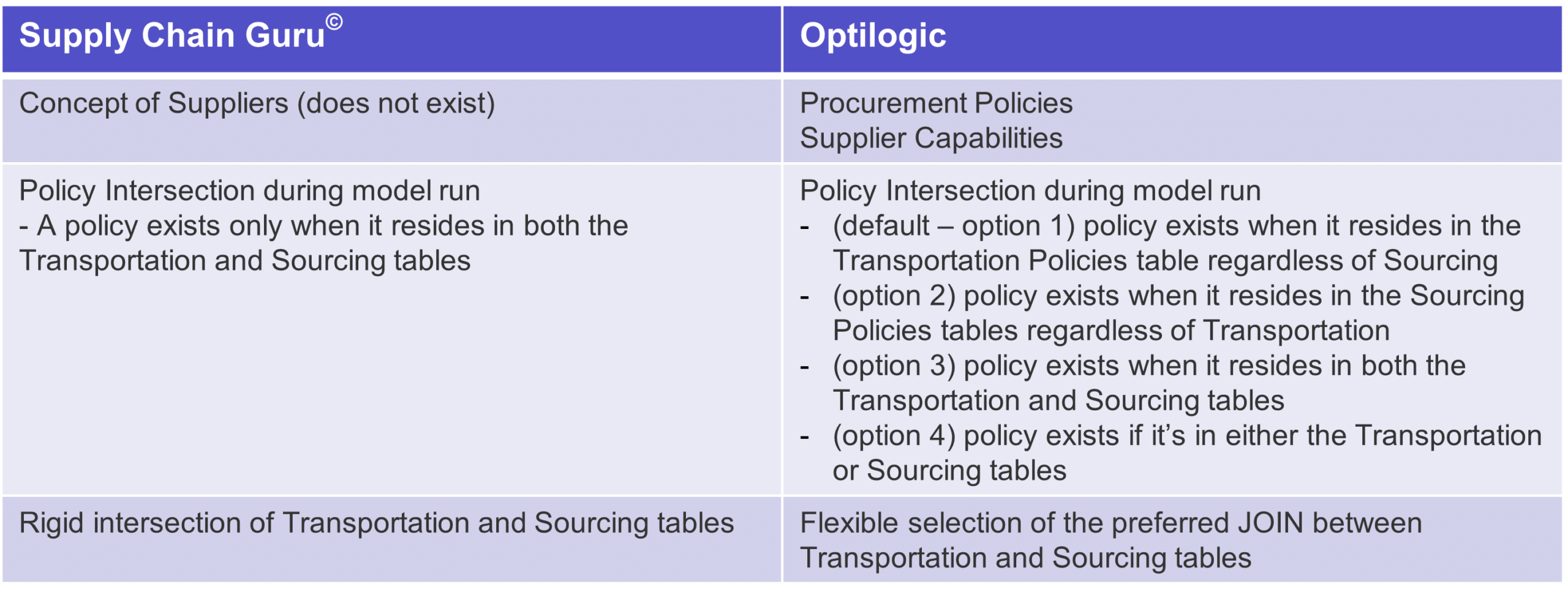
Have you ever wanted to put a site in your model and distinguish whether you owned the site or not? Have you ever wanted to make clear what you own and what you outsource? If so, the suppliers tables are for you:
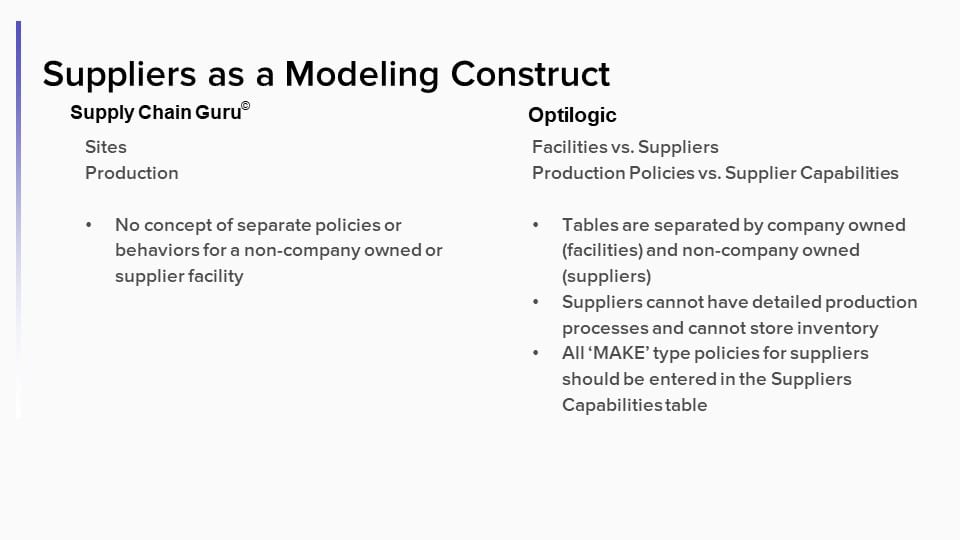
Do you really need a corresponding transportation policy for every sourcing policy and vice versa? Did you know that by doing so you actually making the model take longer to build and solve? Have you ever built a model that was infeasible because you forgot to add a policy?
We put the power in you, the user’s, hands. Simply change the lane creation rule and you can ensure that your model builds and solves the way you want.
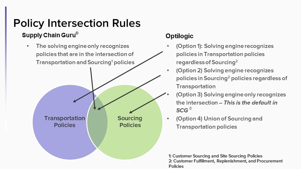
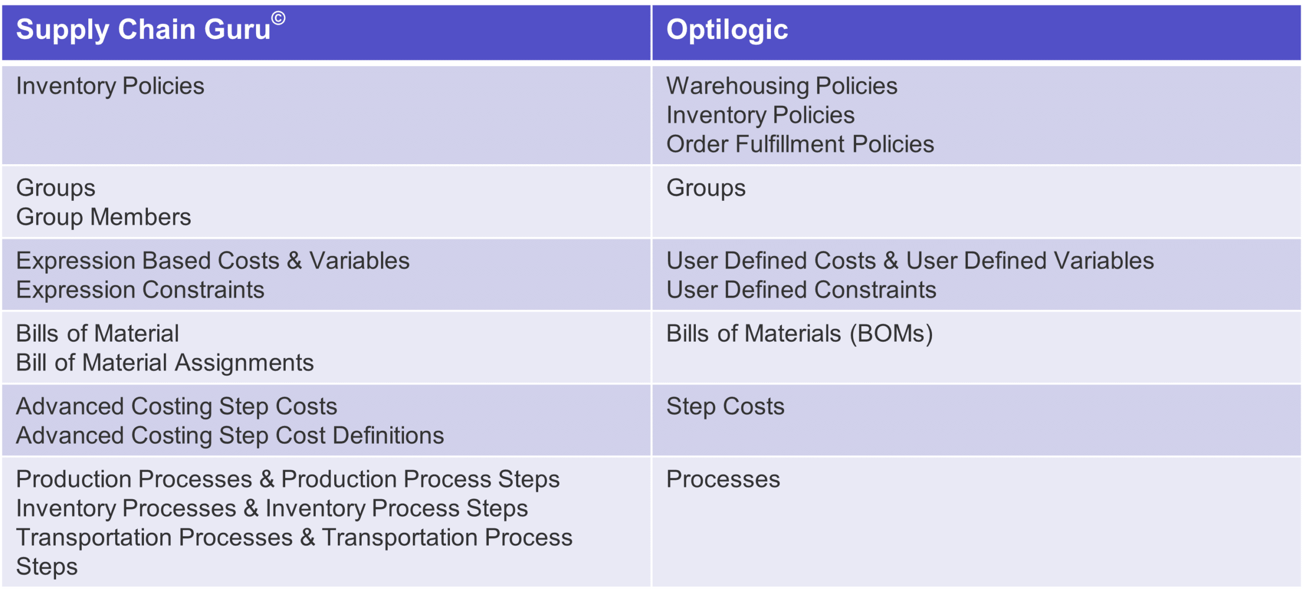
We split inventory policies into three sections because we believe there is a lot going on when you process how to model inventory in your models, especially when you process inventory in simulation. Other than that, we cleaned up the table structure, why enter data in multiple tables if you don’t need to? Where possible we streamlined the table structure to make it easier to enter your data.
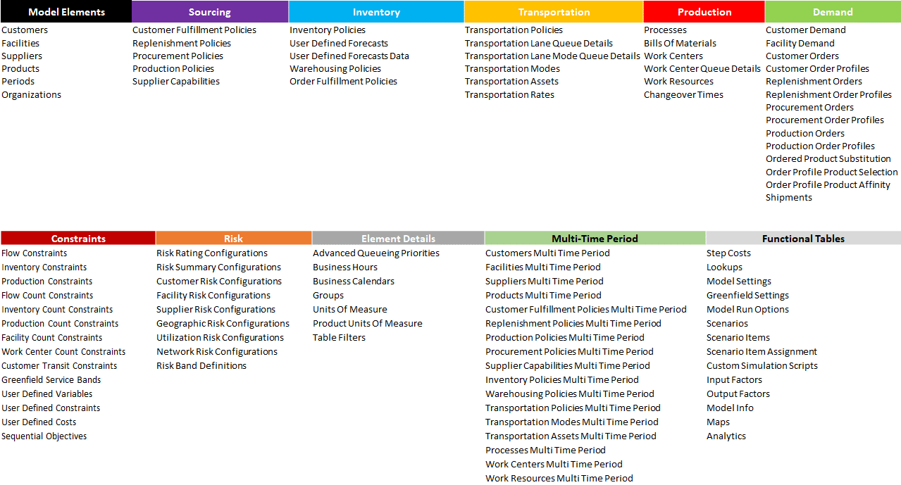
The Anura data model contains 11 categories of tables. The most basic of models can be built by only populated six tables (Customers, Facilities, Products, Customer Demand, Production Policies, and Transportation Policies); however, most models require a few tables from each modeling category to build out a realistic interpretation of the supply chain.
Tables are grouped into the following sections:
With the 2.8 version of Anura there are quite a few new tables and columns being added, along with a small number of existing columns that have been renamed. These updates enable new features including, but not limited to, the following:
We will cover the 2 instances of breaking changes below, followed by a more detailed review of schema adjustments specific to each solver. If you have any questions regarding these updates, please do not hesitate to reach out to support@optilogic.com for further information.
2.7_TransportationRates
The Transportation Rates table previously used by NEO has been renamed to Transportation Band Costing in 2.8. This is done to allow for a Hopper-specific table to be built out and take the name of Transportation Rates. All data upgrades will be processed automatically, but any ETL workflows that targeted the Transportation Rates table in 2.7 will need to be updated.
2.7_OptimizationCostToServeParentInformationReport
Optimization Cost To Serve Parent Information Report has had the CurrentNodeName and ParentNodeName renamed to CurrentSiteName and ParentSiteName. All upgrades will be handled automatically, but any dashboards or external data visualizations that target these columns would need to be updated.
If you are running into issues loading Atlas or Cosmic Frog initially where the loading spinner is stuck on the screen you can attempt to perform a hard refresh of the browser. This spinner being stuck can be caused by the website loading a stale token and refreshing the page without loading from cache should generate a fresh token.
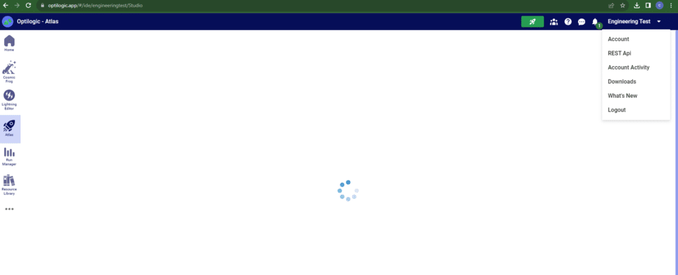
To perform a hard refresh of the browser hit CTRL + F5. Alternatively, you can hit the refresh button in the browser while holding down CTRL.
If the issue persists, please reach out to support@optilogic.com.
Watch the video to learn how to create, manage and hyperscale scenarios:
Model constraints allow us to capture real-world limitations in our supply chain. These limitations might include production capacity, transportation restrictions, storage limits, etc.
By default, Cosmic Frog allows us to incorporate the following constraint types for Neo optimization models:
Each set of constraints has its own table in the Cosmic Frog data schema.

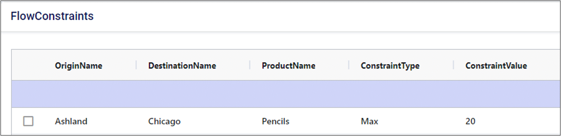
Flow Constraints introduce a limit on the amount of flow (product) that can pass between an origin/destination pair in our supply chain.
In the example below, we limit the number of pencils that the Ashland production site can ship to the Chicago customer to a maximum of 20 per period.
Note that we can adjust the unit of measure of our constraints as needed. For example, we might be interested in limiting the total weight of product shipped between locations, instead of the total count of product.
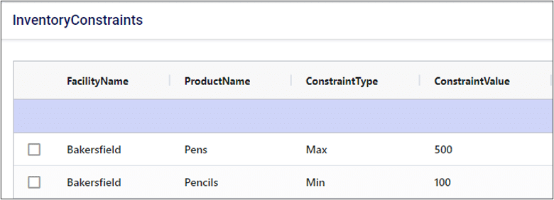
Inventory constraints limit the amount of product that can be stored at a facility. They can represent both minimum and maximum inventory limits.
In the example below we limit the capacity of the Bakersfield distribution center such that it can hold at most 500 pens. We are also requiring that the DC stores at least 100 pencils.
Production constraints limit the amount of product a supplier or a production facility can produce. Like inventory constraints, you can set both minimum and maximum production limits.
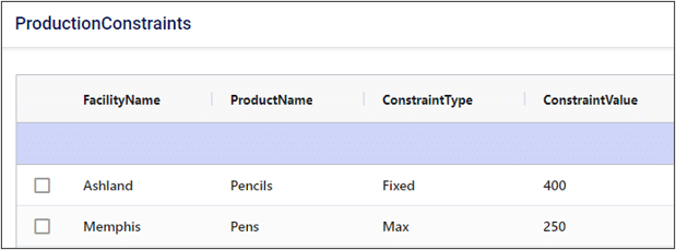
In the example below, the Memphis production can produce at most 250 pens in each period. Additionally, the Ashland site has a fixed production constraint, which requires it to always produce exactly 400 pencils in each period.
Facility count constraints limit the number of facilities that can be used in a Cosmic Frog model. These constraints are often used in facility location and selection problems.
For many of the “count” constraints, we want to apply our constraint across a number of different supply chain elements (e.g. across all facilities). To do this, the group functionality of Cosmic Frog is particularly useful, and often necessary. For more detailed information on using groups in constraints, see Using Groups to Write Model Constraints.
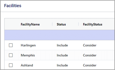
In the following example we want to design a supply chain with exactly 2 facilities, and we want to know the optimal location of these 2 facilities. First, we set the status of candidate locations in our Facilities table to “consider”. Without making this change, our model will be forced to include all facilities where Status = “Include” in our network.
Then, we create a constraint requiring the model to select exactly 2 facilities from the “ProductionSites” group.

Flow count constraints limit the number of flows of a particular product. Flow count constraints are particularly useful in problems where the available transportation resources are limited.
In the following example we are implementing a “single-sourced” rule where each customer is served by exactly one production site. For each customer (enumeration) we look across all production sites (aggregation) and set the flow count to be exactly 1.

Production count constraints allow us to manage the number of product types that are produced at different facilities.
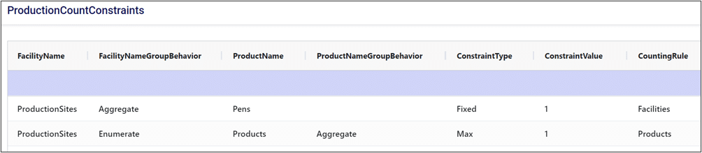
In the example below we add two production count constraints. First, we require that only one production site produces pens. Second, we require that each production site makes at most one product from the “Products” group.
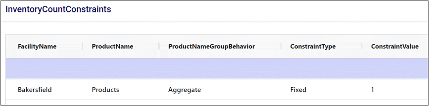
Inventory count constraints allow us to limit the number of product types that are stored at our facilities. In the example below we require the Bakersfield DC to hold at most one type of product.
Custom Columns can be added to any input table directly through Cosmic Frog. To add a custom column to a table, open the table and then select Grid > Create Custom Column
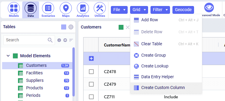
This will open a window on the right-hand side of the screen where you can configure your custom column. Each of the required entries are used as follows:
This will be the name of the custom column. Please note that column names will only be allowed to contain alphanumeric characters and underscores. Spaces are not allowed in column names, and you will not be able to create a column name that begins with a number. If you enter any sort of an invalid column name, you will not be able to save the column and a message will be displayed noting the issues with the name currently entered.
Pseudo typing allows for the data entered into this column to accept all sorts of input formatting without strictly adhering to the Data Type selected for the custom column. For example, if the Data Type for a given custom column is set to numeric and you attempt to import a string into the field, Pseudo Typed = TRUE will allow for this import to succeed. If Pseudo Typed = FALSE, then this import would fail as the field would only accept numbers. This also applies for editing the field within the grid directly.
For reference, all fields within the standard Anura schema are pseudo typed. We will allow for all entries into the data fields and then cast the entries to their appropriate data type for use within maps, dashboards and the application of scenario items.
Select one of the available data types that the data in your custom column will be formatted in. Depending on the selection chosen for the Pseudo Typed setting, this data type will be strictly enforced (Pseudo Typed = FALSE) or be relaxed and only used when generating visuals or applying scenario items (Pseudo Typed = TRUE).
This setting informs Cosmic Frog if the custom column should be used as a primary key for the table when evaluating file imports. If True, the custom column will be included in addition to the table’s default primary key columns.
When data is imported into a Cosmic Frog model through the Import File action, data is loaded using Upsert logic. This means that rows which already exist in a table will be updated, and rows which do not exist will be inserted. Existing rows will be identified using the table’s primary key – all input tables have a preconfigured set of columns that represent the primary key of the input table. For information on which columns represent the primary key of any given table, please reference Downloadable Anura Data Structure – Inputs | Optilogic.
Once all of the settings have been filled out, click Save and your table will refresh with the custom column now being displayed on the far-right of the table. You’ll notice that the column name has been down cased – this is done to align with standard naming convention for PSQL.
If any issues arise during the Custom Column creation, please reach out to support@optilogic.com for further assistance.