As you continue to work with the tool you might find yourself asking, what do these engine names mean and how the heck did they come up with them?
Anura, the name of our data schema, comes from the biological root where Anura is the order that all frogs and toads fall into.
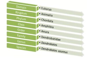
NEO, our optimization engine, takes its name from a suborder of Anura – Neobatrachia. Frogs in this suborder are known to be the most advanced of any other suborder.
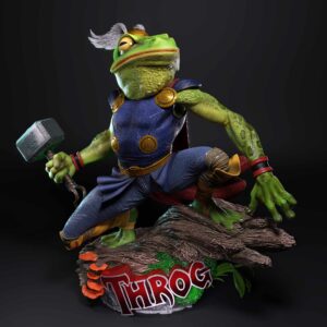
THROG, our simulation engine, takes its name from a superhero hybrid that crosses Thor with a frog (yes, this actually exists)
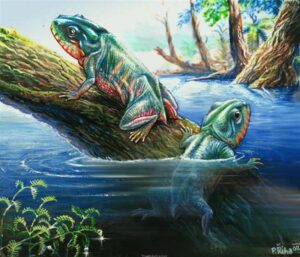
Triad, our greenfield engine, takes its name from the oldest known species of frogs – Triadobatrachus. You can think of it as the starting point for the evolution of all frogs, and it serves as a great starting point for modeling projects too!
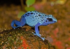
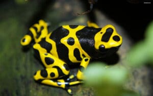
Dart, our risk engine, takes its name from the infamous poison dart frog. Just as you would want to be aware of a poisonous frog’s presence, you’ll also want to be sure to evaluate any opportunities for risks to present themselves.
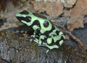
Dendro, our simulation evolutionary algorithm, takes its name from what is known to be the smartest species of frog – Dendrobates auratus. These frogs have the ability to create complex mental maps to evaluate and better navigate their surroundings.
Hopper, our transportation routing engine, doesn’t have a name rooted in frog-related biology but rather a visual of a frog hopping along from stop to stop just as you might see with a multi-drop transportation route.

There can be many different causes for an ODBC connection error, this article contains a couple of specific error messages along with resolution steps.
Resolution: Please make sure that the updated PSQL driver has been installed. This can be checked through your ODBC Data Sources Administrator
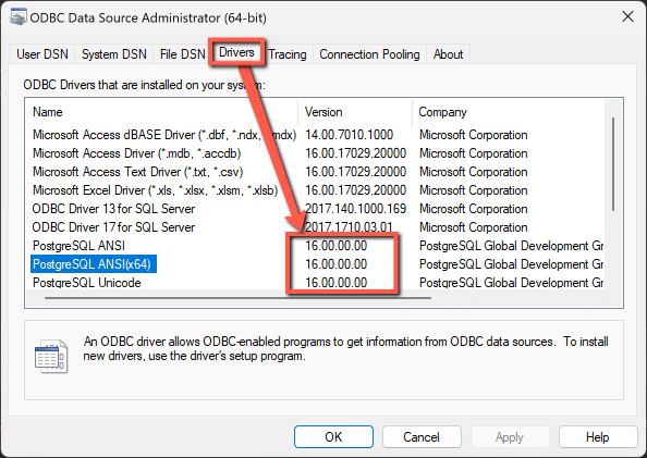
Latest versions of the drivers are located here: https://www.postgresql.org/ftp/odbc/releases/ from here, click on the latest parent folder, which as of June 20, 2024 will be REL-16_00_0005. Select and download the psqlodbc_x64.msi file. When installing, use the default settings from the installation wizard.
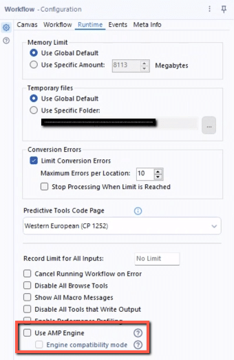
Resolution: Please confirm the PSQL drivers are updated as shown in the previous resolution. If this error is being thrown while running an Alteryx workflow specifically, please disable the AMP Engine for the Alteryx workflow.
Running a model is simple and easy. Just click the run button and watch your Python model execute. Watch the video to learn more.
To leverage the power of hyperscaling, click the “Run as Job” button.
Running a model from Atlas via the SDK requires the following inputs:
Model data can be stored in two common locations:
1. Cosmic Frog model (denoted by a .frog suffix) stored within Postgres SQL database in the platform
2. .CSV files stored within Atlas
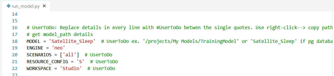
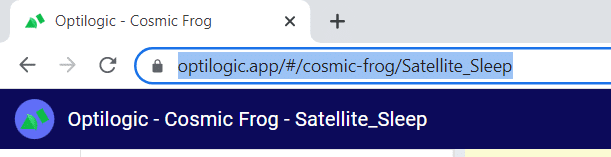
For #1 simply enter the database name within single quotes. For example to run a model called Satellite_Sleep I will need to enter this data in the run_model.py file
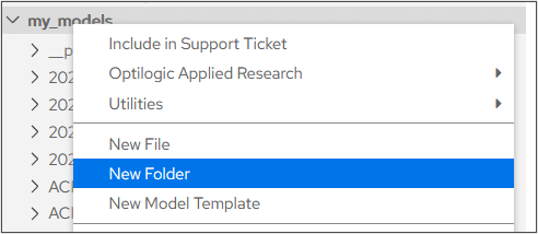
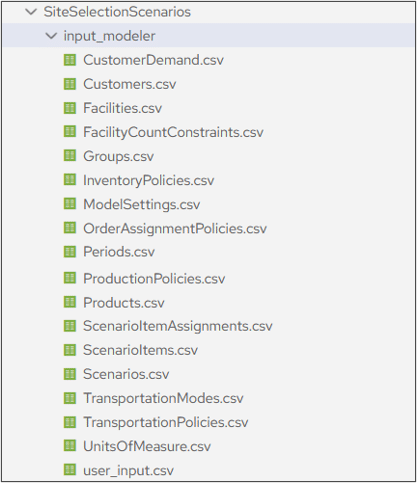
For #2 you will need to create a folder within Atlas to store your .CSV modeling files:
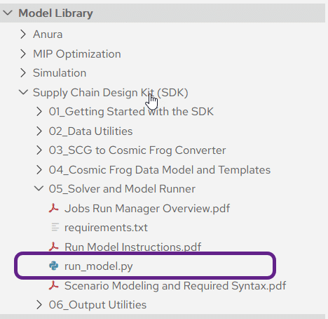
Each Atlas account is loaded with a run_model.py file located within the SDK folder in your Model Library
Double click the file to open it within Atlas and enter the following data:
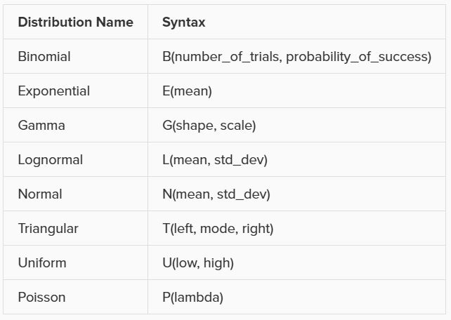
Several input columns used by Throg (Simulation) will accept distributions as inputs. The following distributions, along with their syntax, are currently supported by Throg:
A user-defined Histogram is also supported as an acceptable input. These will be defined in the Histograms input table, and to reference a histogram in an allowed input column simply put in the Histogram Name.
The data for our visualizations comes from our Cosmic Frog model database. This is often stored in the cloud using a unique identifier.

We can decide if we want to use Optilogic servers to do our data computations, or if we want the computations to be performed locally.

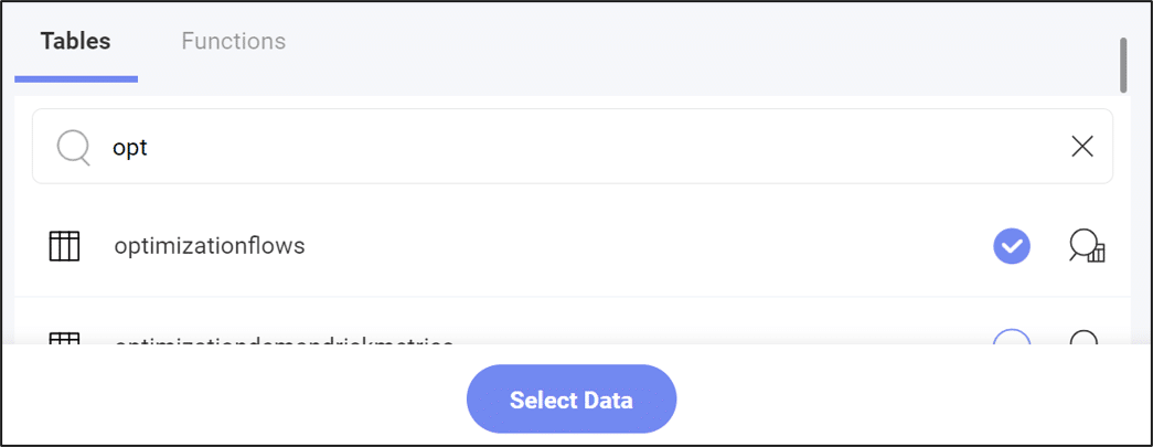
Next, we must decide which table we want to use for our visualization. Generally, the results of running our model are stored in the “optimization” tables, so it can be helpful to use search for this to see output data. However, we can also use tables containing input data if desired.
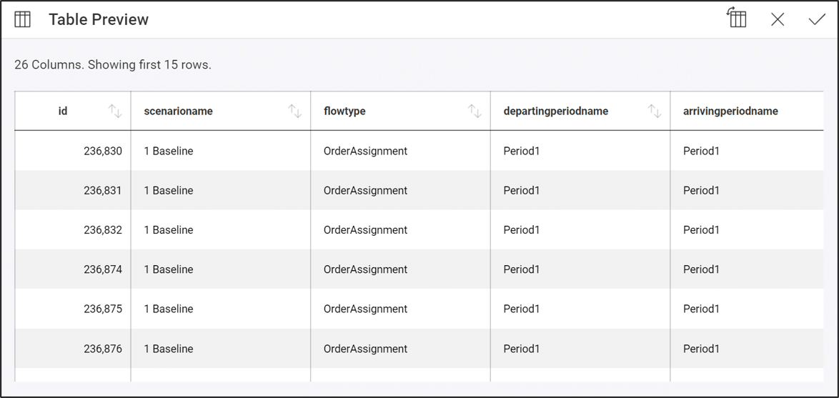
We can also preview the data in a table using the magnifying glass button:

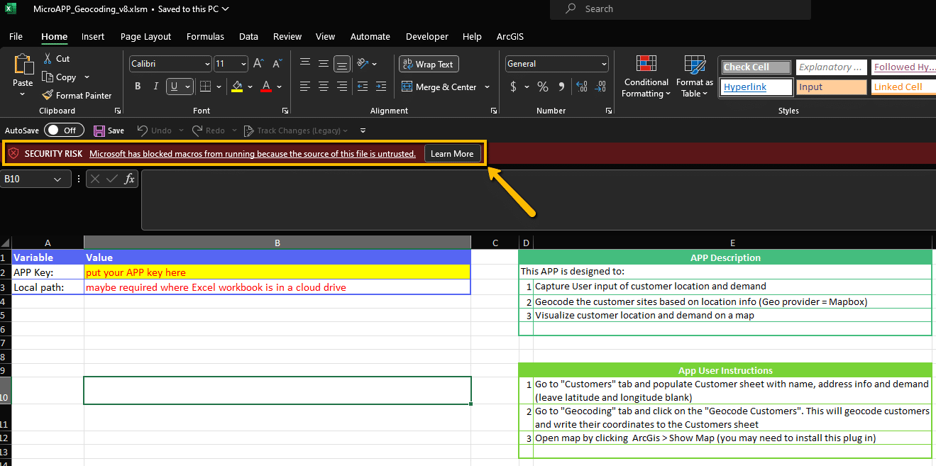
When downloading all of the related files for any of the sample Excel Apps that are posted to our Resource Library, you will likely encounter macro-enabled Excel workbooks (.xlsm) which might have their macros disabled following download.
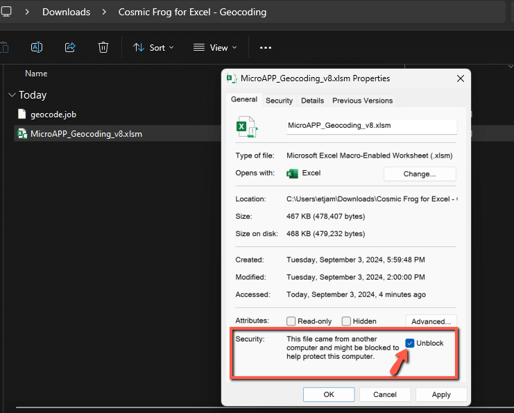
To enable the macros, you can right-click on the Excel file in a File Explorer and select the option for Properties. In the Properties menu, check the box in the Security section to Unblock the file and then hit Apply.
You can then re-open the document and should see the macros are now enabled.
Some of the Excel templates also make use of add-ins to help expand the workbook’s capabilities. An example of this is the ArcGIS add-in which allows for map visuals to be created directly in the workbook. It is possible that these add-ins might be disabled by default in the Microsoft Office settings, if that is the case you should see an error message as follows:
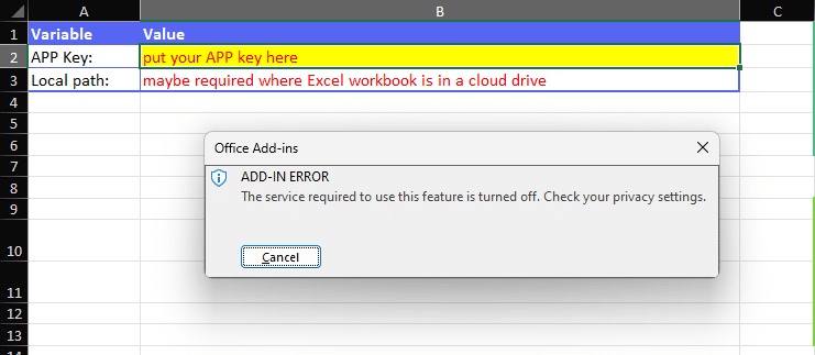
This can be resolved by updating your Privacy Settings under your Microsoft Office Account page. To access this menu, click into File > Account > Account Privacy > Manage Settings. You will then want to make sure that in the Optional Connected Experiences, the option to Turn on optional connected experiences is enabled.
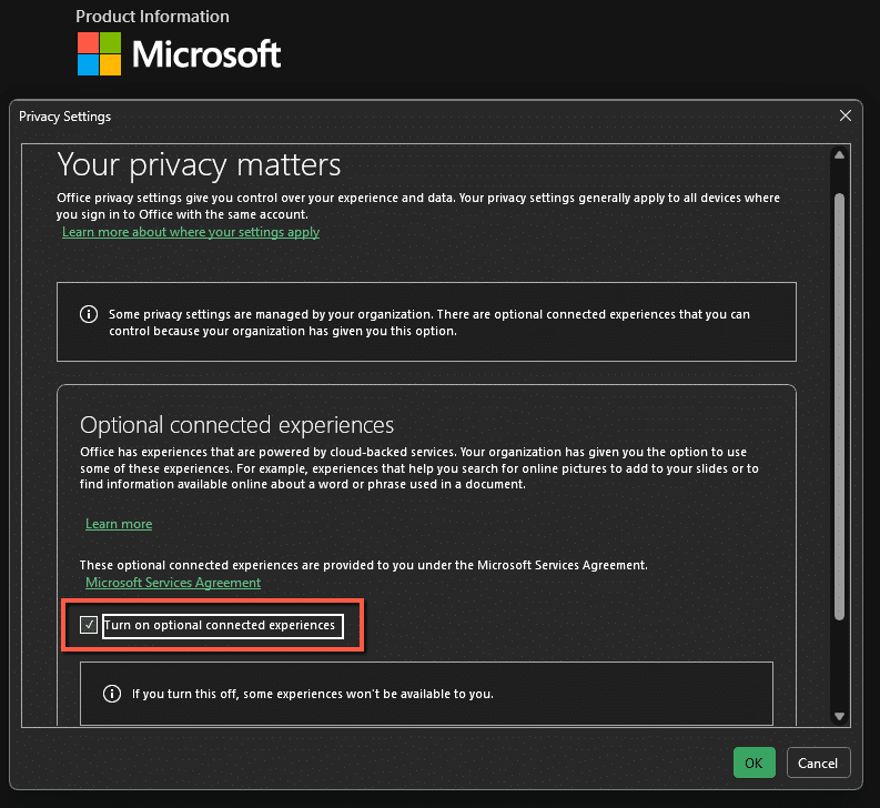
Updating this value will require a restart of Microsoft Office. Once the restart is completed, you should see that the add-ins are now enabled and working as expected.
If other issues come from any Resource Library templates please do not hesitate to reach out to support@optilogic.com.
Please find a list of model errors that might appear in the Job Error Log and their associated resolutions.
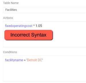
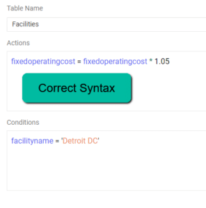
Resolution – Please check to see if a scenario item was built where an action does not reference a column name. Scenario Actions should be of the form ColumnName = …..
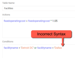
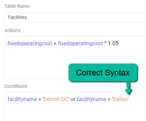
Resolution – Please check to see if there is a string in the scenario condition that is missing an apostrophe to start or close the string
Resolution – This indicates an intermittent drop in connection when reading / writing to the database. Re-running the scenario should resolve this error. If the error persists, please reach out to support@optilogic.com.
‘Connection Info’ is required when connecting 3rd party tools such as Alteryx, Tableau, PowerBI, etc. to Cosmic Frog.
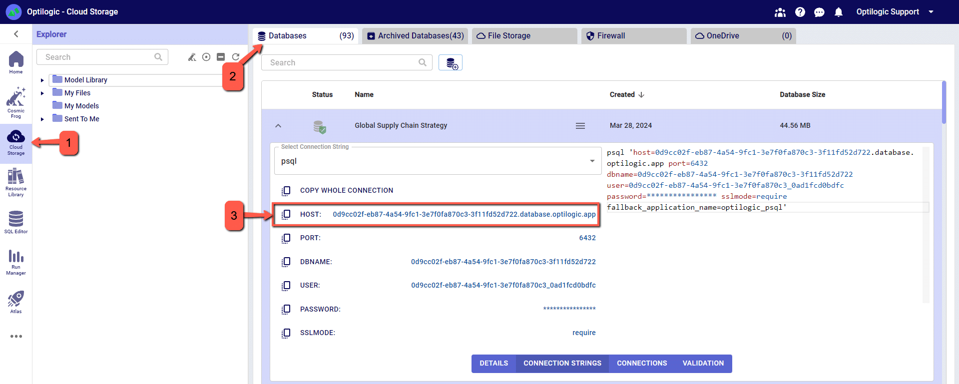
Anura version 2.7 makes use of Next-Gen database infrastructure. As a result, connection strings must be updated to maintain connectivity.
Severed connections will produce an error when connecting your 3rd party tool to Cosmic Frog.
Steps to restore connection:
Cosmic Frog ‘HOST’ value can be copied from Cloud Storage browser.
The following instructions begin with the assumption that you have data that you wish to upload to your Cosmic Frog model.
The instructions below assume the user is adding information to the Suppliers table in the model database. This will use the same connection that was previously configured to download data from the Customers table.
Drag the “Output Data” action into the Workflow and click to select “Write to File or Database”
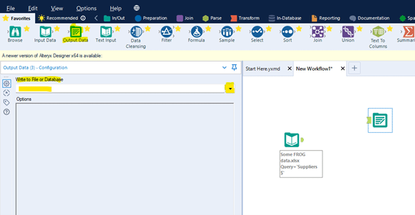
Select the relevant ODBC connection established earlier, in this example we called the connection “Alteryx Demo Model.”

You will be prompted to enter a valid table name to which the data will be written in the model database. In this example enter suppliers (all in lower case to match the table name in PostGres, which is case sensitive).
Click OK

Within the Options menu – edit “Output Options” to Append Existing in the drop-down list.
Within the Options menu – edit “Append Field Map” by clicking the three dots to see more options.
Select “Custom Mapping” option and then use the drop-down lists to map each field in the Destination column to the Source column. Fields of the same name, but case sensitive as it is PostGres.
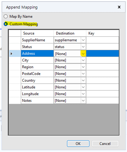
Click OK
Now you can Run the Workflow to upload the data to your model. Once it has completed check the Suppliers table in Cosmic Frog to see the data.
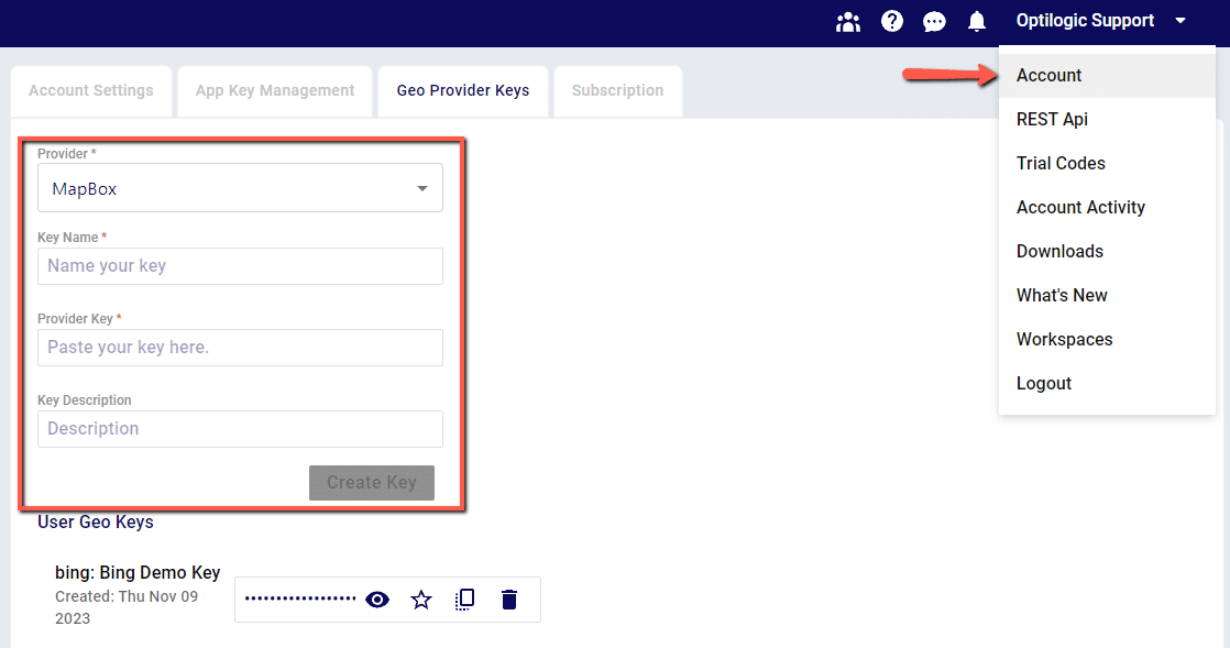
By default, the Geocoding option in Cosmic Frog will use Mapbox as the geodata provider. Other supported providers will be Bing, Google, PTV and PC Miler. If you have an access key for an alternate provider and would like to configure this provider as the default option, follow these two steps:
1. Set up your geocoding key under your Account > Geoprovider Keys page
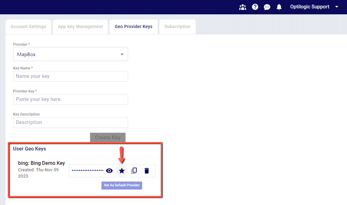
2. Once a new key has been created, set the key as the Default Provider to be used by clicking the Star icon next to the key. This key will now be used for Geocoding in Cosmic Frog
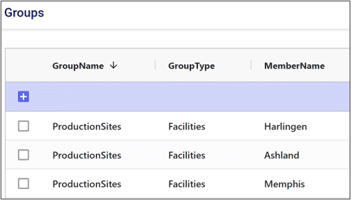
Adding model constraints often requires us to take advantage of Cosmic Frog’s Groups feature. Using the Groups table, we can define groups of model elements. This allows us to reference several individual elements using just the group name.
In the example below, we have added the Harlingen, Ashland, and Memphis production sites to a group named “ProductionSites”.
Now, if we want to write a constraint that applies to all production sites, we only need to write a single constraint referencing the group.
When we reference a group in a constraint, we can choose to either aggregate or enumerate the constraint across the group.
If we aggregate the constraint, that means we want the constraint to apply to some aggregate statistic representing the entire group. For example, if we wanted the total number of pens produced across all production sites to be less than a certain value, we would aggregate this constraint across the group.
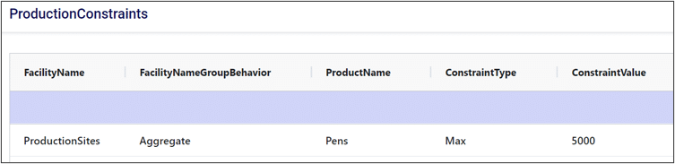
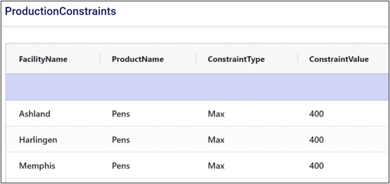
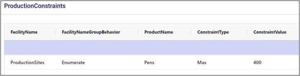
Enumerating a constraint across a group applies the constraint to each individual member of the group. This is useful if we want to avoid writing repetitive constraints. For example, if each production site had a maximum production limit of 400 pens, we could either write a constraint for each site or write a single constraint for the group. Compare the two images below to see how enumeration can help simplify our constraint tables.
Without enumeration:
With enumeration:
Thank you for using the most powerful Supply Chain Design software in the galaxy (I mean, as far as we know).
To see the highlights of the software please watch the following video.
The team at Optilogic has built a powerful tool to take existing Supply Chain Guru models from either a .scgm or .mdf format and convert them to the Optilogic Anura and .frog schema.
To try this feature click the three dots on the right side of your Home Screen to select SCG Converter icon.
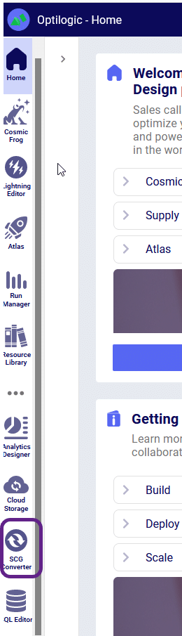
This will take you to the converter page:
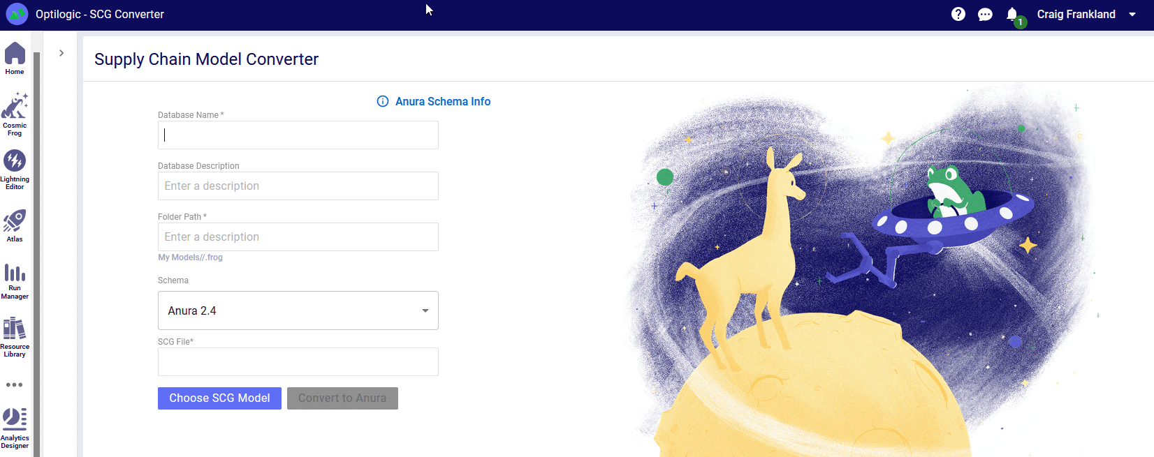
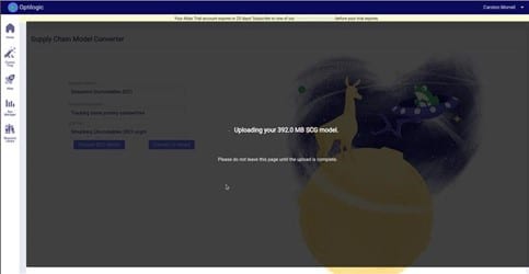
From here you will need to name your model and select the model you wish to convert. Then you will able to click the “Convert to Anura” button. Please do not click away from the browser tab as the model is uploading. After the upload is complete you will be redirected to another page while the model is converted to the Anura schema. At this time it is safe to click away from the page as your conversion will be in process.
Once the conversion is complete you will be redirected to the SQL Editor page where you can start executing queries on your new Anura database! You will notice that there are two schemas in the database: _original_scg and anura_2_8.
You can review the data from the original database under the _original_scg tables and can see the new transformed data under the anura_2_8 tables. You will also find a new table in the anura schema called ‘scg_conversion_log’ – this table will provide logging information from the conversion process to track where data transformations outside of the default schema took place, and will also note any warnings or issues that the converter ran into. A full list of column mappings can be found here.
For a review of Conditions related to Scenarios please refer to the article here. Conditions, in Scenarios, take the form of a comparison that can create a filter in your table structure.
If you are ever doubting the name of a column that needs to be used in an action, you can type CTRL+SPACE to have the full list of columns available to you displayed. Alternatively, you can start typing and the valid column names will auto-complete.
Standard comparison operators include: =, >, <, >=, <=, !=. You can also use the LIKE or NOT LIKE operators and the % or * values for wildcards for string comparisons. The % and * wildcard operators are equivalent within Cosmic Frog (though, best practice is to use the % wildcard symbol since this is valid in the database code). If you have multiple conditions, the use of AND / OR operators are supported. The IN operator is also supported for comparing strings.
Cosmic Frog will color code syntax with the following logic:
Following are some examples of valid condition syntax:
To describe the action and conditions of our scenario, there are specific syntax rules we need to follow.
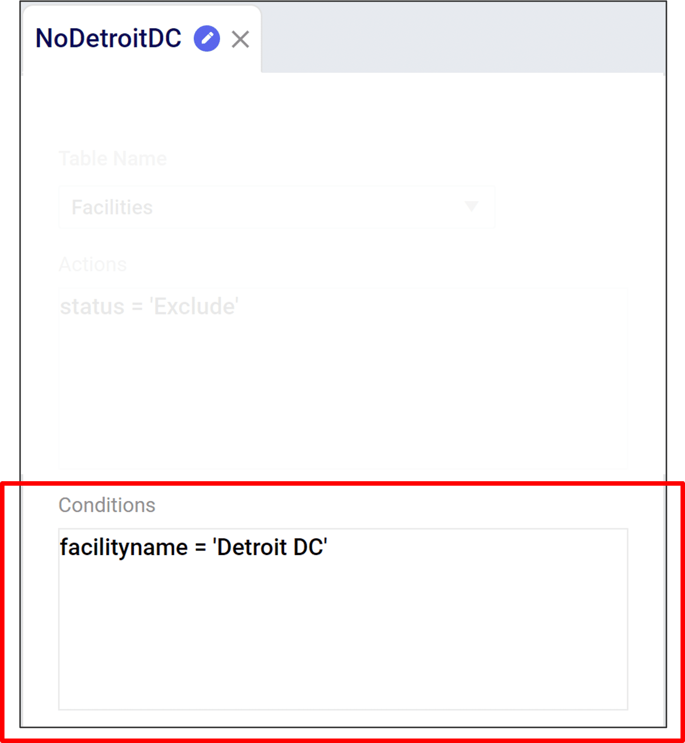
In this example, we are editing the Facilities table to define a scenario without a distribution center in Detroit.
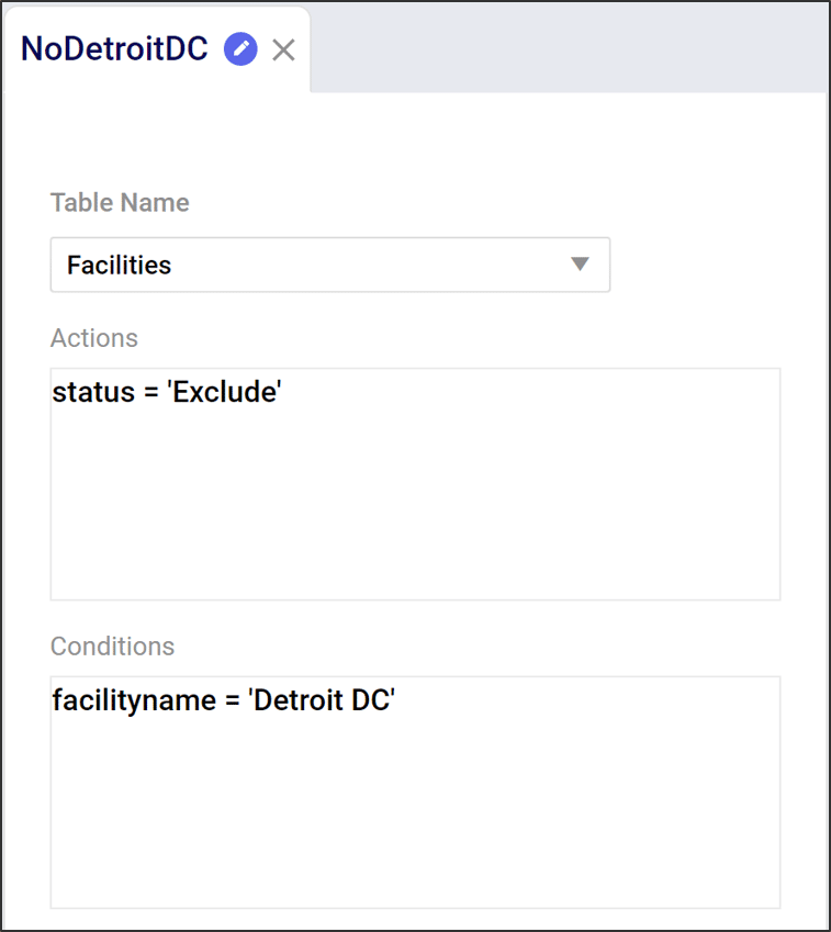
Actions describe how we want to change a table. Actions have 2 components:
Writing actions takes the form of an equation:
Further detail on action syntax can be found here.
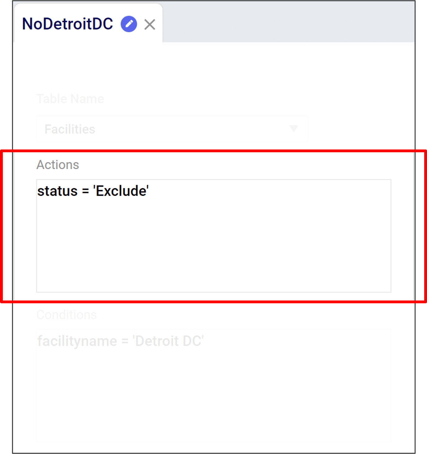
Conditions describe what we want to change. They are Boolean (i.e. true/false) statements describing which rows to edit. Conditions have 3 components:
Conditions take the form of a comparison, such as:
Further detail on Conditions syntax can be found here.
For a review of Actions related to Scenarios please refer to the article here. Writing actions take the form of an equation:
If you are ever doubting the name of a column that needs to be used in an action, you can type CTRL+SPACE to have the full list of columns available to you displayed. Alternatively, you can start typing and the valid column names will auto-complete.
When assigning numerical values to a column, we can use mathematical operators such as +, -, *, and /. Likewise you can use parenthesis to establish a preferred order of operations. Below are some examples of the syntax.
When assigning numerical values to a column we can use mathematical operators such as +, -, *, and /. Likewise you can use parentheses to establish a preferred order of operations as shown in the following examples.
When assigning string values to a column you must use single quotation marks to reference any string that is not a column name. Some examples of changing values with a string are included in the examples below:
For a detailed walk-through of all map features, please see the "Getting Started with Maps" Help Center article.
You can edit and filter the information shown in a map layer by utilizing the Layer Menu on the right hand side of your map screen. This menu opens when a layer is selected and contains the following tabs:
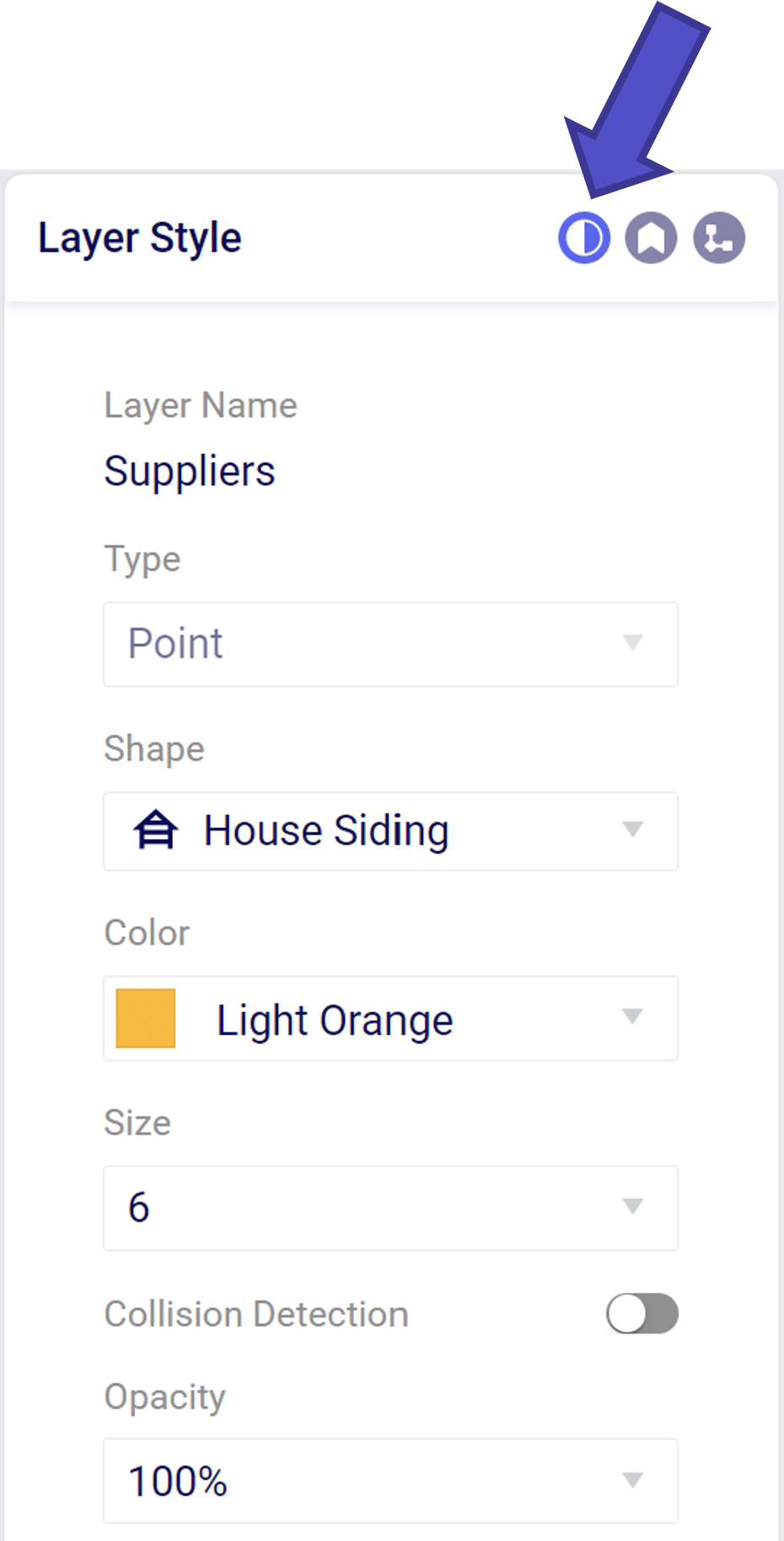
From the layer style menu we can modify how the layer will appear on the map
From the layer label menu we can add text descriptors the map layer.
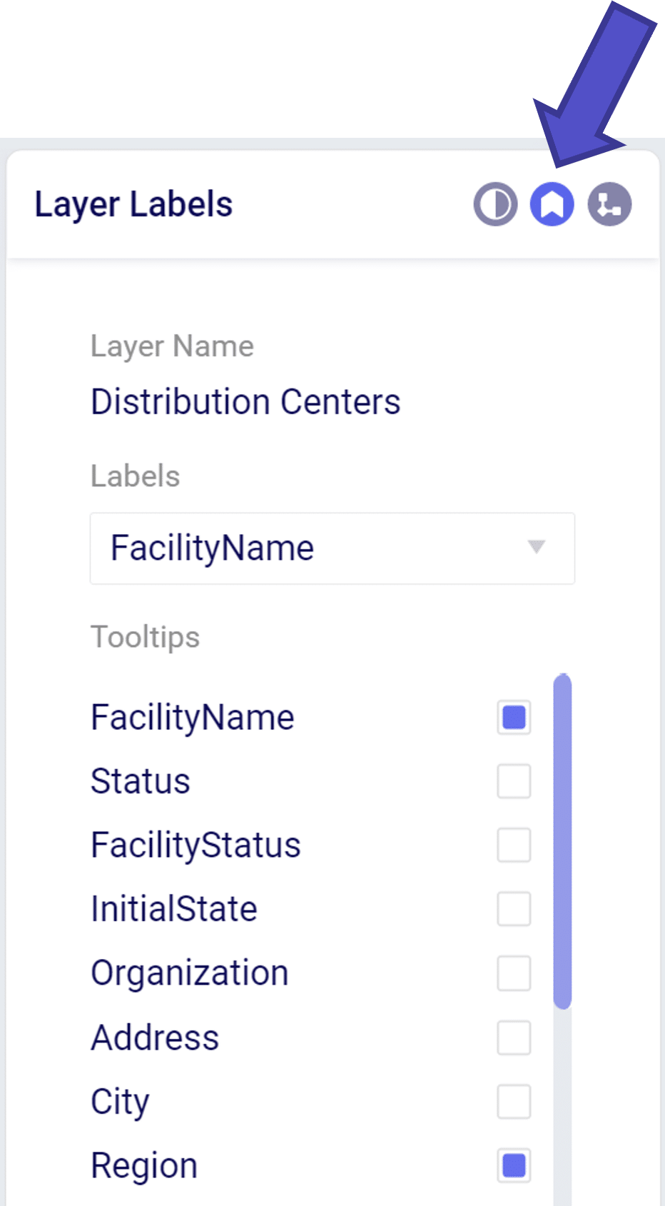
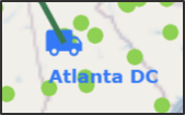
The “Labels” dropdown menu allow you to add a text descriptor next to a layer item. Only one item may be selected in the label dropdown.
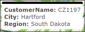
The “Tooltip” is a floating box that appears when hovering over a layer element. We can add/remove items displayed in the tooltip by selecting in the “Tooltips” menu.
The Condition Builder menu allows you to edit the data included in your layer. The most important item is to select the Table Name using the drop down menu that you wish to show on the map. This can include point items like Customers or Facilities or transportation arcs like OptimizationFlowSummary.
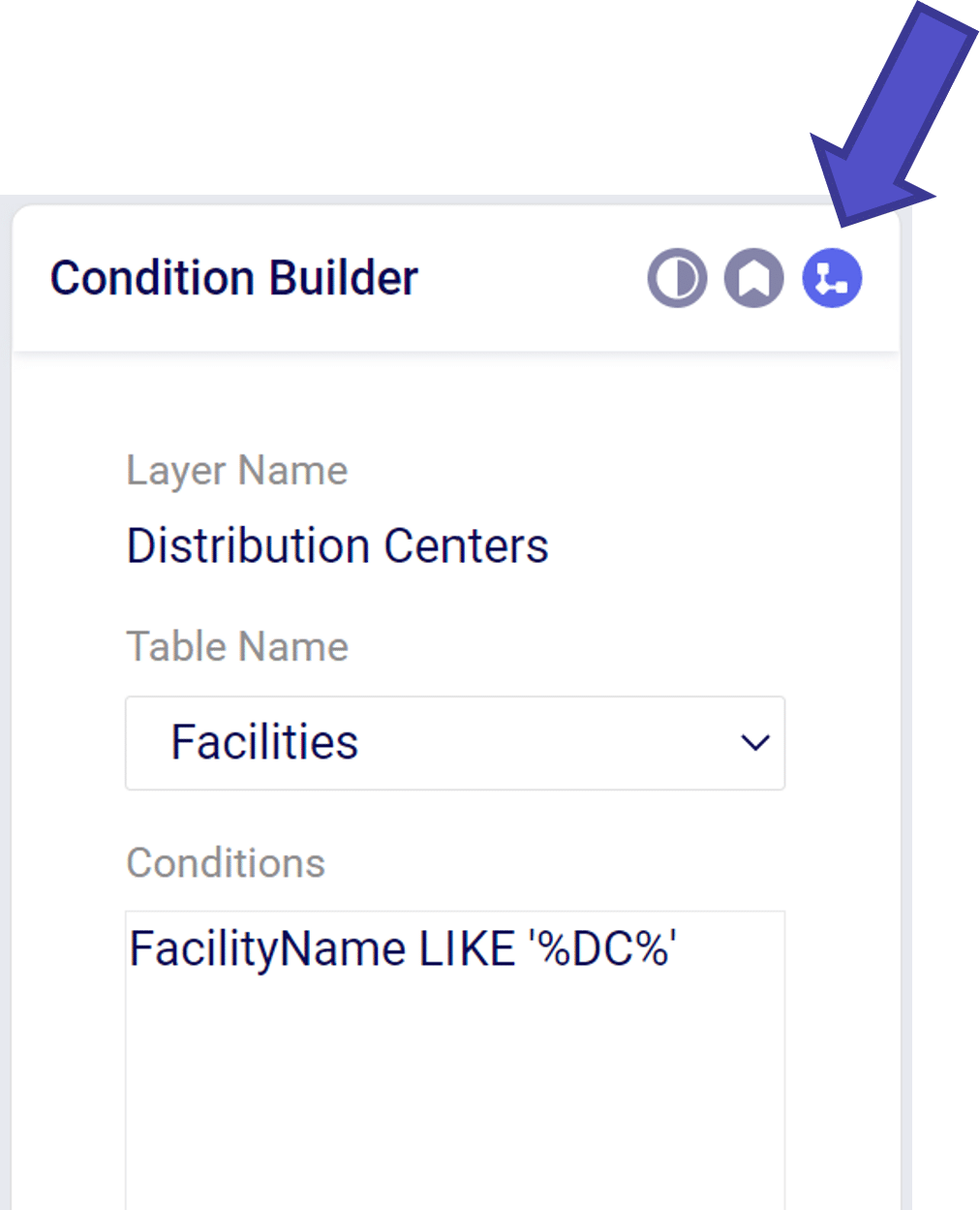
Within the Condition Builder you can use conditions to filter the table further to a subset of the data in the table. The filter syntax is similar to the syntax used when creating scenarios.
These instructions assume you have already made a connection to your database as described in Connecting to Optilogic with Alteryx.
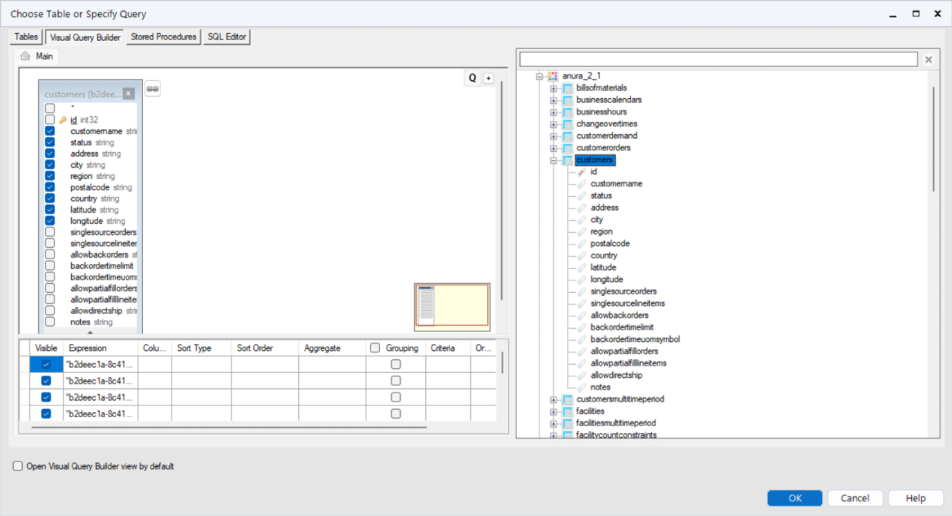
Once connected you will see the schemas and tables in the Cosmic Frog database. In this case we will select some columns from the Customers table. Drag and drop the tables required to the left hand “Main” pane. Click the columns required. Click OK.
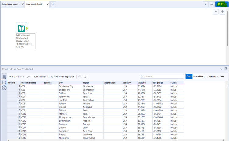
At this point you can run your workflow and it will be populated with the data from the connected database.
Being able to assess the Risk associated with your supply chain has increasingly become more important in a quickly changing world with high levels of volatility. Not only does Cosmic Frog calculate an overall supply chain risk score for each scenario that is run, but it also gives you details about the risk at the location and flow level, so you can easily identify the highest and lowest risk components of your supply chain and use that knowledge to quickly set up new scenarios to reduce the risk in your network.
By default, any Neo optimization, Triad greenfield or Throg simulation model run will have the default risk settings, called OptiRisk, applied using the DART risk engine. See also the Getting Started with the Optilogic Risk Engine documentation. Here we will cover how a Cosmic Frog user can set up their own risk profile(s) to rate the risk of the locations and flows in the network and that of the overall network. Inputs and outputs are covered and in the last section notes & tips & additional resources are listed.
The following diagram shows the Cosmic Frog risk categories, their components, and subcomponents.
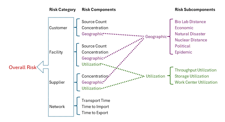
A description of these risk components and subcomponents follows here:
Custom risk profiles are set up and configured using the following 9 tables in the Risk Inputs section of Cosmic Frog’s input tables. These 9 input tables can be divided into 5 categories:
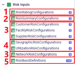
Following is a summary of these table categories; more details on individual tables will be discussed below:
We will cover some of the individual Risk Input tables in more detail now, starting with the Risk Rating Configurations table:

In the Risk Summary Configurations table, we can set the weights for the 4 different risk components that will be used to calculate the overall Risk Score of the supply chain. The 4 components are: customers, facilities, suppliers, and network. In the screenshot below, customer and supplier risk are contributing 20% each to the overall risk score while facility and network risk are contributing 30% each to the overall risk score.
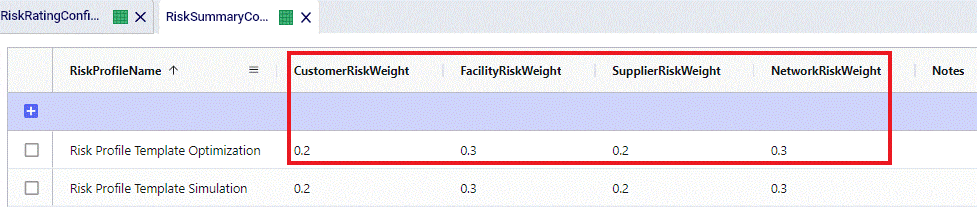
These 4 weights should add up to 1 (=100%). If they do not add up to 1, Cosmic Frog will still run and automatically scale the Risk Score up or down as needed. For example, if the weights add up to 0.9, the final Risk Score that is calculated based on these 4 risk categories and their weights will be divided by 0.9 to scale it up to 100%. In other words, the weight of each risk category is multiplied by 1/0.9 = 1.11 so that the weights then add up to 100% instead of 90%. If you do not want to use a certain risk category in the Risk Score calculation, you can set its weight to 0. Note that you cannot leave a weight field blank. These rules around automatically scaling weights up or down to add up to 1 and setting a weight to 0 if you do not want to use that specific risk component or subcomponent also apply to the other “… Risk Configurations” tables.
Following are 2 screenshots of the Facility Risk Configurations table on which the weights and risk bands to calculate the Risk Score for individual facility locations are specified. A subset of these same risk components is also used for customers (Customer Risk Configurations table) and suppliers (Supplier Risk Configurations table). We will not discuss those 2 tables in detail in this documentation since they work in the same way as described here for facilities.


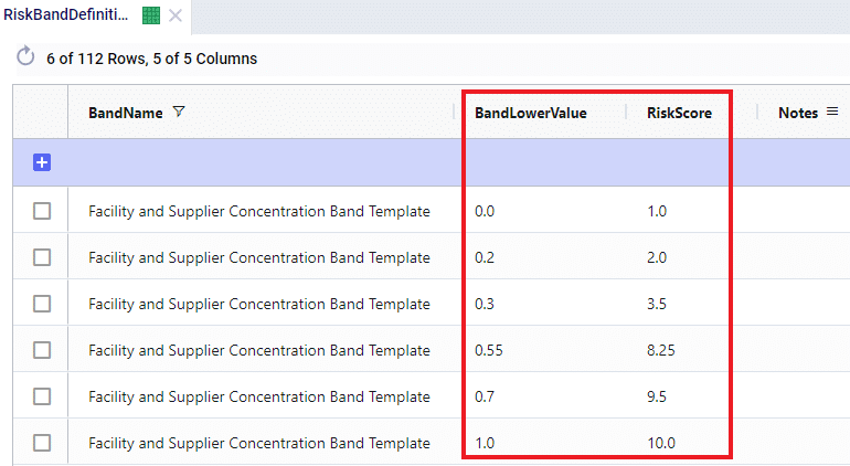
The first band is from 0.0 (first Band Lower Value) to 0.2 (the next Band Lower Value), meaning between 0% and 20% of total network throughput at an individual facility. The risk score for 0% of total network throughput is 1.0 and goes up to 2.0 when total network throughput at the facility goes up to 20%. For facilities with a concentration (= % of total network throughput) between 0 and 20%, the Risk Score will be linearly interpolated from the lower risk score of 1.0 to the higher risk score of 2.0. For example, a facility that has 5% of total network throughput will have a concentration risk score of 1.25. The next band is for 20%-30% of total network throughput, with an associated risk between 2.0 and 3.5, etc. Finally, if all network throughput is at only 1 location (Band Lower Value = 1.0), the risk score for that facility is 10.0. The risk scores for any band run from 1, lowest risk, to 10, highest risk.
Following screenshot shows the Geographic Risk Configurations table with 2 of its risk subcomponents, biolab distance and economic:

As an example here in the red outline, the Biolab Distance Risk is specified by setting its weight to 0.05 or 5% and specifying which band definition on the Risk Band Definitions table should be used, which is “BioLab and Nuclear Distance Band Template”. The Definition of this band template is as follows when looked up in the Risk Band Definitions table:
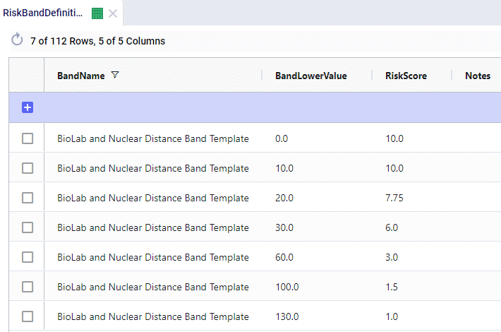
This band definition says that if a location is within 0-10 miles to a Biolab of Safety Level 4, the Risk Score is 10.0. A distance of 10-20 miles has an associated Risk Score between 10 and 7.75, etc. If a location is 130 miles or farther from a biolab of safety Level 4, the Risk Score is 1.0.
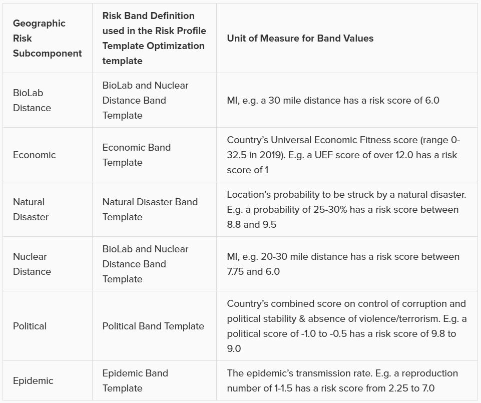
The other 5 subcomponents of Geographic Risk are defined in a similar manner on this table: with a Risk Weight field and a Risk Band field that specifies which Band Definition on the Risk Band Definitions table is to be used for that risk subcomponent. The following table summarizes the names of the Band Definitions used for these geographic risk subcomponents and what the unit of measure is for the Band Values with an example:
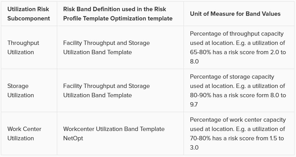
Similar to the Geographic Risk component, the Utilization Risk component also has its own table, Utilization Risk Configurations, where its 3 risk subcomponents are configured. Again, each of the subcomponents has a Risk Weight field and a Risk Band field associated with it. The following table summarizes the names of the Band Definitions used for these utilization risk subcomponents and what the unit of measure is for the Band Values with an example:
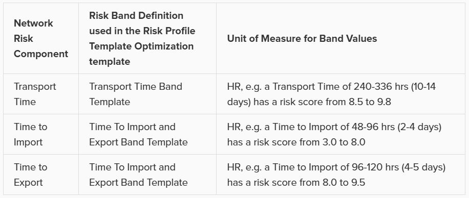
Lastly on the Risk Inputs side, the Network Risk Configurations table specifies the components of Network Risk in a similar manner: with a Risk Weight and a Risk Band field for each risk component. The following table summarizes the names of the Band Definitions used for these network risk subcomponents and what the unit of measure is for the Band Values with an example:
Risk outputs can be found in some of the standard Output Summary Tables and in the risk specific Output Risk Tables:

The following screenshot shows the Optimization Risk Metrics Summary output table for a scenario called “Include Opt Risk Profile”. It shows both the OptiRisk and Risk Rating Template Optimization risk score outputs:

On the Optimization Customer Risk Metrics, Optimization Facility Risk Metrics, and Optimization Supplier Risk Metrics tables, the overall risk score for each customer, facility, and supplier can be found, respectively. They also show the risk scores of each risk component, e.g. for customers these components are Concentration Risk, Source Count Risk, and Geographic risk. The subcomponents for Geographic risk are further detailed in the Optimization Geographic Risk Metrics output table, where for each customer, facility, and supplier the overall geographic risk score and the risk scores of each of the geographic risk subcomponents are listed. Similarly, on the Facility Risk Metrics and Supplier Risk Metrics tables, the Utilization Risk score will be listed for each location, whilst the Optimization Utilization Risk Metrics table will detail the risk scores of the subcomponents of this risk (throughput utilization, storage utilization, and work center utilization).
Let’s walk through an example of how the risk score for the facility Plant_France_Paris_9904000 was calculated using a few screenshots of input and output tables. This first screenshot shows the Optimization Geographic Risk Metrics output table for this facility:

The geographic risk score of this facility is calculated as 4.0 and the values for all the geographic risk subcomponents are listed here too, for example 8.2 for biolab distance risk and 3.6 for political risk. The overall geographic risk of 4.0 was calculated using the risk score of each geographic risk subcomponent and the weights that are set on the Geographic Risk Configurations input table:

Geographic Risk Score = (biolab distance risk * biolab distance risk weight + economic risk * economic risk weight + natural disaster risk * natural disaster risk weight + nuclear distance risk * nuclear distance risk weight + political risk * political risk weight + epidemic risk * epidemic risk weight) / 0.8 = (8.2 * 0.05 + 5.3 * 0.2 + 2.8 * 0.3 + 2.3 * 0.05 + 3.6 * 0.1 + 4.5 * 0.1) / 0.8 = 4.0. (We need to divide by 0.8 since the weights do not add up to 1, but only to 0.8).
Next, in the Optimization Facility Risk Metrics output table we can see that the overall facility risk score is calculated as 6.8, which is the result of combining the concentration risk score, source count risk score, and geographic risk score using the weights set on the Facility Risk Configurations input table.

This screenshot shows the Facility Risk Configurations input table and the weights for the different risk components:

Facility Risk Score = (geographic risk * geographic risk weight + concentration risk * concentration risk weight + source count risk * source count risk weight) / 0.6 = 4.0 * 0.3 + 9.3 * 0.2 + 10.0 * 0.1) / 0.6 = 6.8. (We need to divide by 0.6 since the weights do not add up to 1, but only to 0.6).
A few things about Risk in Cosmic Frog that are good to keep in mind:
For a detailed walk-through of all map features, please see the "Getting Started with Maps" Help Center article.
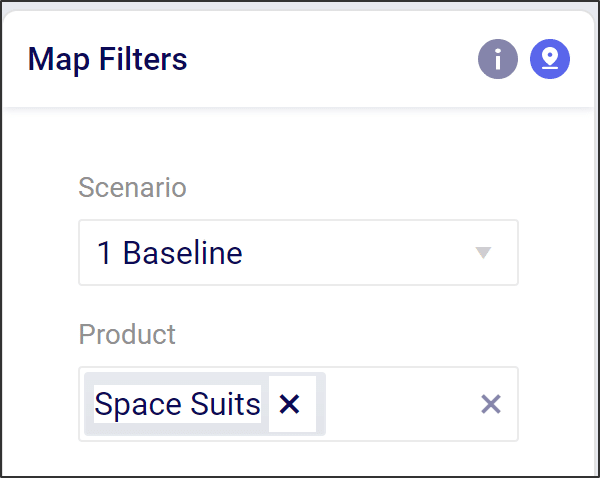
You can edit and filter the base data located with a map using the Map Filter menu. This menu opens when the map name is highlighted or selected. From here you are able to select the following items to be shown in the map:
Note: leaving the product filter blank will include all products in the model
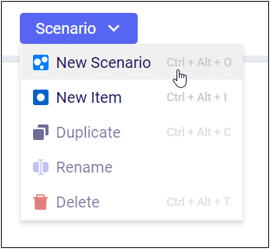
To create a scenario you need to do three things:
From the Scenario tab in Cosmic Frog select the blue button called “Scenario” and click on “New Scenario.”
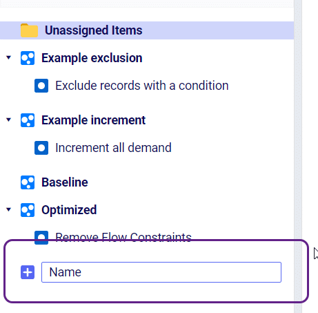
Type the name of the scenario you would like to create in the panel window.
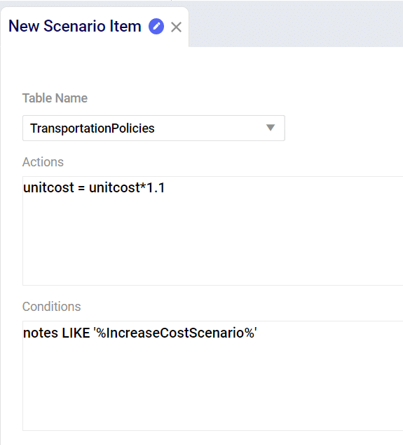
From the same drop down as “New Scenario” select “New Item” to create a scenario item. Enter the name of your scenario item in the window. After you press enter the Scenario Item window will be active where you will select the following:
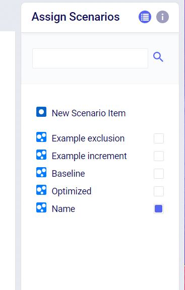
After you have created and saved the Scenario Item you need to assign that item to a scenario. On the right hand side of your screen there is a table called “Assign Scenarios.” From here you can check/uncheck the Scenarios where you wish to use the new Scenario Item.
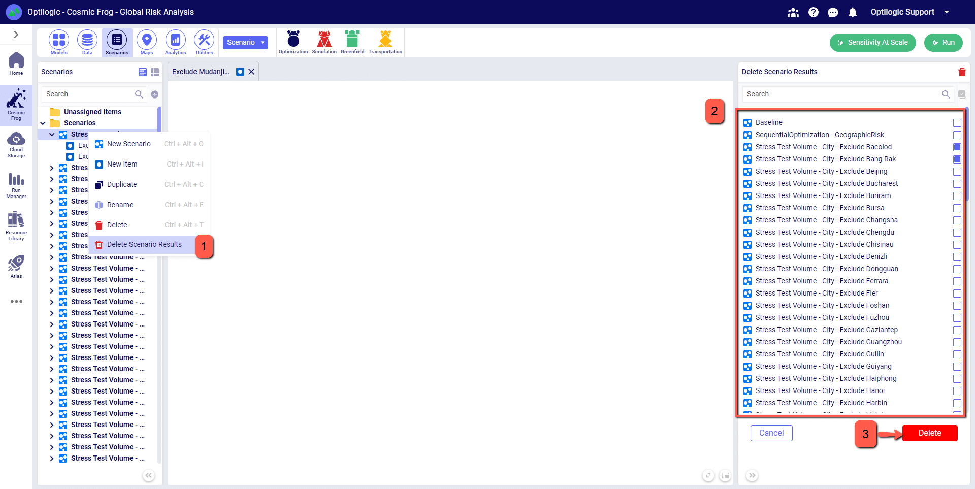
You can clear output data from all model output tables in one quick action. Navigate to the Scenarios tab and from the scenario drop-down menu select the Delete Scenario Results option. This can also be accessed by right-clicking on any scenario name. Next, from the window on the right-hand side of the screen you can select the scenario(s) that you want to delete output data for. Once selected, click the Delete button and all output data will be cleared for the selected scenarios.
Anura contains 100+ (and growing) input tables to organize modeling data.
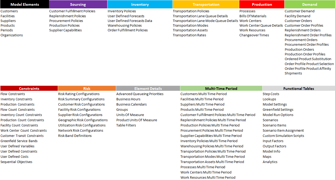
There are six minimum required tables for every model:
This includes one table to identify the demand that must be met, two tables to lay out the structure, and a last table to link them all together with policies.
Most supply chain design models use at least one table each of the first five model categories (Modeling Elements, Sourcing, Inventory, Transportation, Demand). A Neo model converted from Supply Chain Guru© will generally contain the following tables:
By entering information in all of these tables you will have successfully added all demand, created all model elements, created sourcing and transportation policies for all arcs, and added an inventory policy to ensure inventory can be stored throughout the supply chain.
While not required, many Neo models will also contain data in the following tables:
The File Explorer is a fully functioning view into your workspace file system. To open the File Explorer, look for the following icon on the left-hand side of the Atlas environment:

To expand a folder to view its contents simply click anywhere on the folder, its label, or the expand icon (the small triangle next to the folder itself).
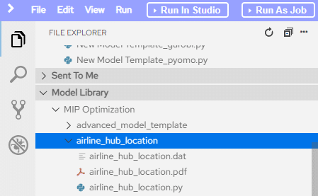
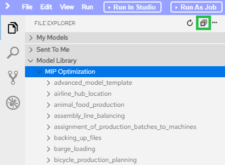
To collapse the folder you can either click on the same area again, or you can collapse all folders by clicking the button outlined below.
To open a file, navigate to it in the file explorer and double-click on it. Once done, the file will load into the editor. Please note that some files will not show properly in the editor, such as files that contain binary content or encrypted content.
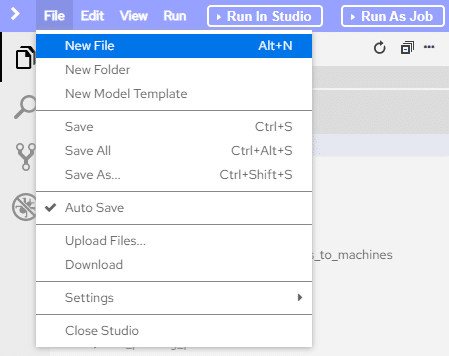
There are two ways you can create a new file; through the file menu:
or via the file explorer context menu.
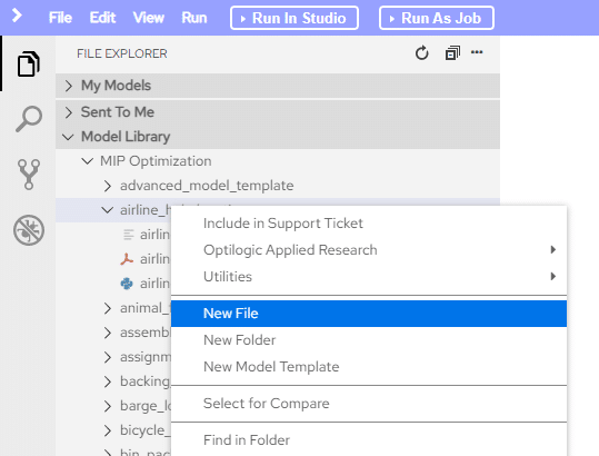
Keep in mind that the context you have selected in the file explorer is where the new folder will go, so if you want the folder underneath a specific other folder make sure to select that folder before you begin. That being said, if you forget you can still move the folder afterward.
To duplicate a file or folder, select the Duplicate command from the right-click context menu. This will create a copy of the file or folder in the same location with the suffix _copy.
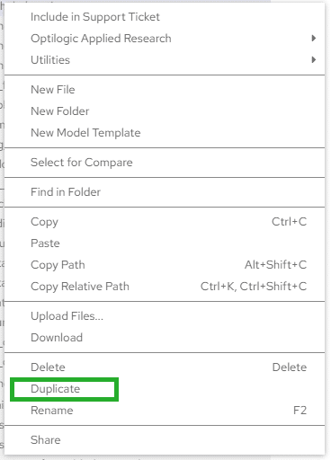
To rename a file or folder, select the Rename command from the right-click context menu or use the hotkey F2 while the file or folder is selected. This will present a dialog where you can type in the new name that you want to use. Once specified, hit Enter or click the OK button to apply the new name.
To upload a file or files, make sure that you have a folder selected. From the right-click context menu select the Upload Files… command or select the same command from the file menu. Select the file or files from the file selection dialog and hit Enter or click the Open button. This will upload the selected files to the folder that you have selected.
To download a file or folder, select the Download command from the right-click context menu or the same command from the file menu. This will download the selected file or folder to your local machine. If you have selected a folder, the contents will be compressed into a .tar archive file. You will need to use a file archiving tool to extract the contents of the archive.
To save a file, select the Save option from the file menu or use the hotkey CTRL+S. This will save the changes in the file that has focus in the editor. Note, a file with focus will have the tab in the editor have the same background as the background of the editor itself. You can tell if a file needs to be saved by the presence of a white dot in the file header open in the editor.
You can delete a file or folder by selecting the Delete command from the right-click context menu or hitting the Delete key on your keyboard.
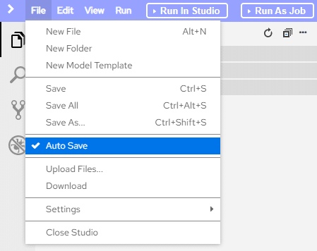
By default, the auto-save option is turned on. This means that your files will automatically save as you are editing them. You can turn this on or off by selecting the Auto Save option in the file menu.
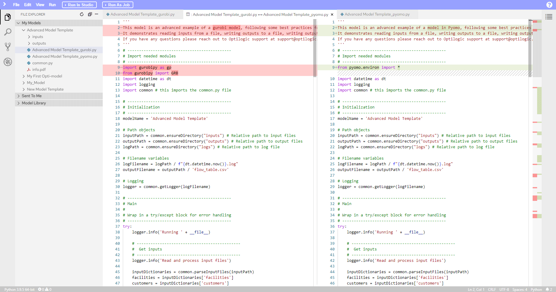
Atlas includes a file comparison tool. This will show you line-by-line differences between two files.
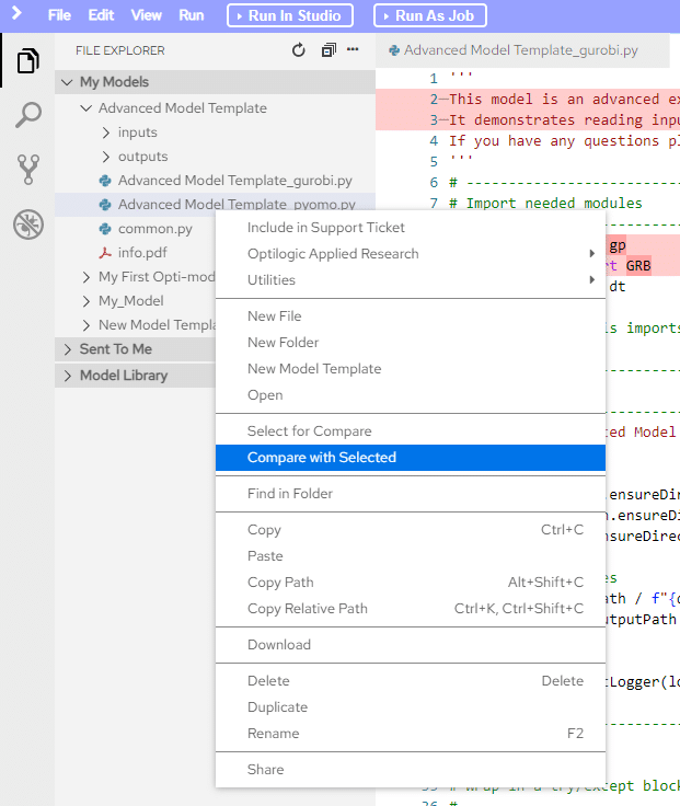
To use it you can either select the Compare with Each Other command from the right-click context menu while two files are selected, or you can select the Select for Compare command on the first file, then select the Compare with Selected command on the other file you would like to compare.
When there are changes to your workspace file system but they haven’t shown up visually, you can refresh the explorer to show you the latest state on disk. This can happen sometimes if the models you are building are writing out files. To refresh the explorer, click the refresh button in the upper right.