If you are comfortable with traditional linear programming techniques, you can select the “Write Input Solver Files” and “Write LP File” parameters to get useful output files.

After running, these files are in your file explorer.
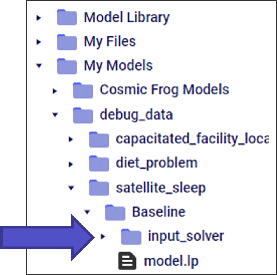
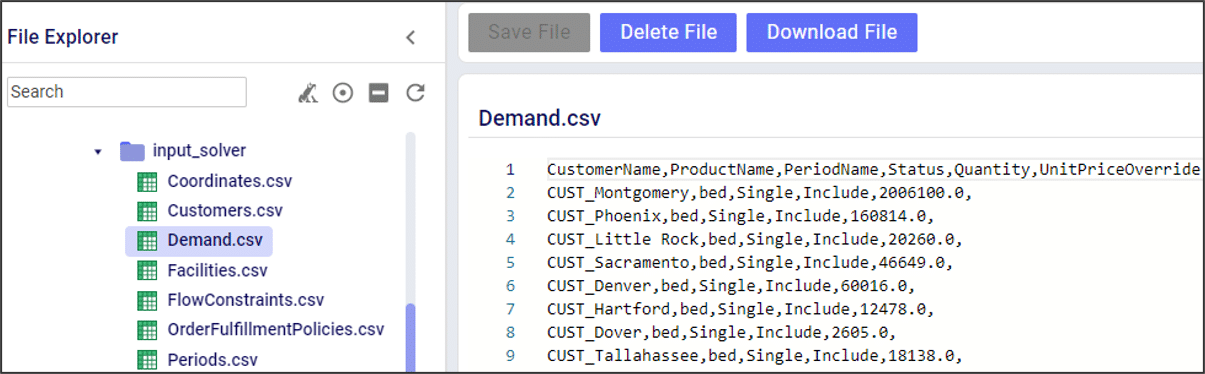
The “input_solver” folder has a list of all the tables that are entered into the optimization solver. This is useful for:
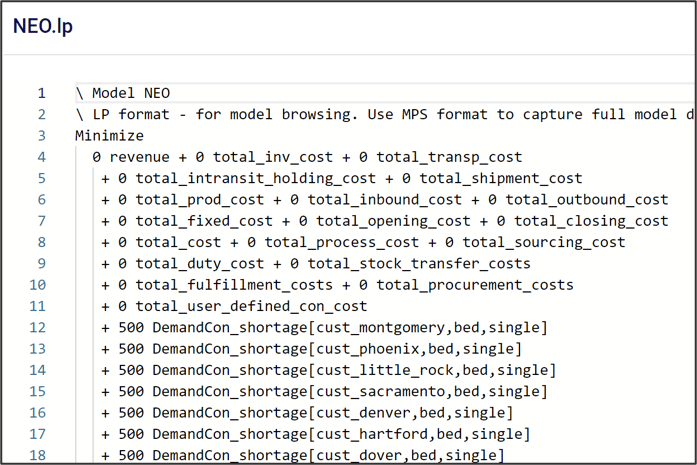
The “model.lp” file shows the model in a more traditional MIP optimization format, including the objective function and model constraints.

When using the Infeasibility Diagnostic engine, the LP file is different than a traditional Neo run. In this case, the cost coefficients in the objective function are set to 0. Instead, a positive cost coefficient is added to each slack constraint, and the goal of the model is to minimize the slack values. This allows us to find the “edge” of infeasibility.
After every Cosmic Frog run, it’s a great habit to check the OptimizationValidationErrorReport table. Even for models that run successfully, this table can have useful information on how the input data is being processed by the solver.
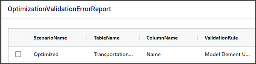
Key columns in the validation error report can tell you:
Validation errors that have “high” or “moderate” severity are likely to cause an infeasible model. In fact, Cosmic Frog has an “infeasibility checker” that looks for these kinds of errors and flags them before running the model to save you run time.
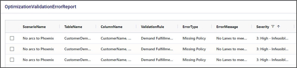
In this example, there are no transportation lanes that can deliver beds to CUST_Phoenix, so demand cannot be fulfilled. The infeasibility checker finds this and stops the model run before it even tries to optimize.


A couple of examples of how we could fix this error:
The OutputValidationErrorReport table is often very useful, even if a model “successfully” runs. This table will catch potential errors that do not cause infeasibility but could change the model results. In this example, there is a typo in the CustomerDemand table for “CUST_Montgomery”. Here, the model drops that row in the demand table. This will not cause an infeasible model, as it just removes that demand constraint. However, it means that no product will be sent to this customer in our optimized result.

This video guides you though creating your free account and the features of the Optilogic Cosmic Frog supply chain design platform.
If you are running into issues receiving your account confirmation email, please see the troubleshooting article linked here.
Greenfield analysis (GF) is a method for determining the optimal location of facilities in a supply chain network. The Greenfield engine in Cosmic Frog is called Triad and this name comes from the oldest known species of frogs – Triadobatrachus. You can think of it as the starting point for the evolution of all frogs, and it serves as a great starting point for modeling projects too! We can use Triad to identify 3 key parameters:
GF is a great starting point for network design—it solves quickly and can reduce the number of candidate site locations in complicated design problems. However, a standard GF requires some assumptions to solve (e.g. single time period, single product). As a result, the output of a Triad model is best suited as initial information for building a more robust Cosmic Frog optimization (Neo) or simulation (Throg) model.
You can run GF in any Cosmic Frog model. Running a GF model only requires two input tables to be populated:

A third important table for running GF is the Greenfield Settings table in the Functional Tables section of the input tables. We call our GF approach “Intelligent Greenfield” because of the different parameters available by configuring this settings table. The Greenfield Settings table is always populated with defaults and users can change these as needed. See the Greenfield Setting Explained help article for an explanation of the fields in this table.
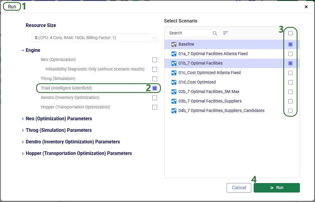
A greenfield analysis starts with clicking the “Run” button at the right top of the Cosmic Frog application, just like a Neo or Throg model.

After clicking on the Run button, the Run screen comes up:
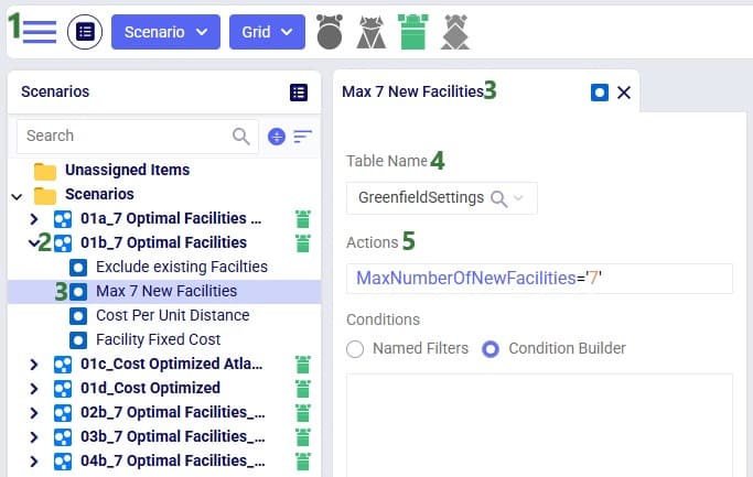
Besides making changes to values in the Customers and/or Customer Demand tables, GF scenarios often make changes to 1 or multiple settings on the Greenfield Settings table. The next screenshot shows an example of this:
To improve the solve speed of a Triad model, we can use customer clustering. Customer clustering reduces the size of the supply chain by grouping customers within a given geometric range into a single customer. We can set the clustering radius (in miles) in the Greenfield Settings table in the Customer Cluster Radius column.

Clustering is optional, and leaving this column blank is the same as turning off clustering.
While grouping customers can significantly improve the run time of the model, clustering may result in a loss of optimality. However, Greenfield is typically used as a starting point for a future Neo optimization model, so small losses in optimality at this phase are typically manageable.
The only constant is change. When building our supply chains, the “optimal” design doesn’t only mean lowest cost. What happens if (or perhaps when) a disruption occurs? Fragile, low-cost supply chains can end up costing more in the long run if they aren’t resilient to the dynamic nature of today’s world.
We believe that optimality includes resilience. That’s why every Cosmic Frog run includes a risk rating from our DART risk engine.
Every Cosmic Frog run outputs an Opti Risk score. The Opti Risk score is an aggregate measure of the overall supply chain risk. It includes the following sub-categories:
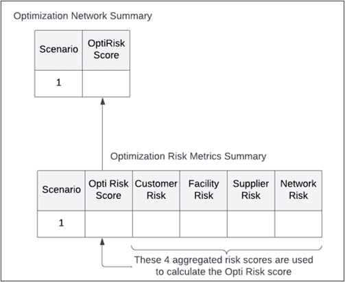
After running a model, you can find the Opti Risk score (as well as the scores for each of the sub-categories) in the output risk tables. The Opti Risk score can also be found in the OptimizationNetworkSummary table.
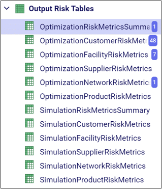
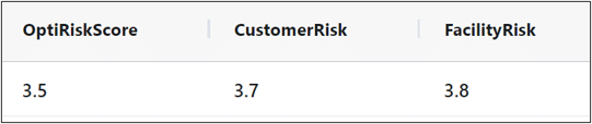
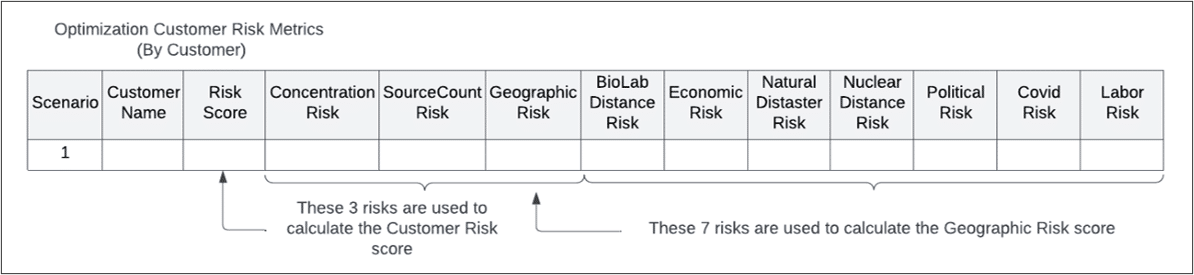
The overall Customer Risk score is an aggregation of each individual customer’s risk described in the OptimizationCustomerRiskMetrics or SimulationCustomerRiskMetrics tables. In each scenario, there is one risk score per customer per period.
Each customer risk score includes:
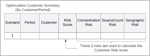
For each sub-category, the geographic risk score is also an aggregation of several risk factors:
Like the customer risk score, the overall facility risk score is an aggregation of risk across all facilities in your supply chain. In the FacilityRiskMetric tables, there is an individual risk score per facility per period.
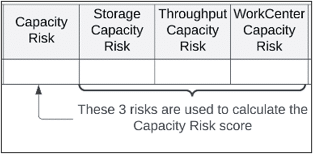
The facility risk score includes:
The capacity risk has three sub-components:
The facility geographic risk has the same components as the customer geographic risk.

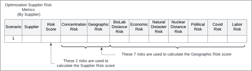
The supplier risk is calculated per supplier per period and includes:
Both the concentration and geographic risks include the same elements as described previously.
Network risk differs from the other risk scores in that it is not tied to a specific supply chain element. There is only one network risk score per scenario, and it includes:
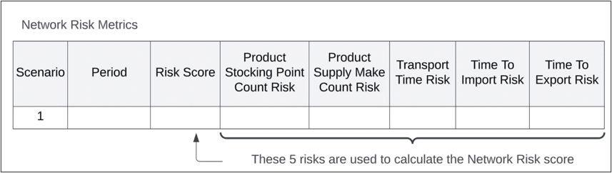
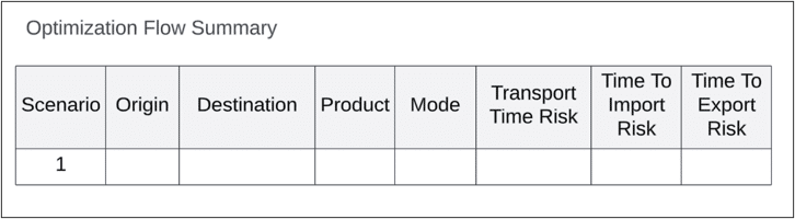
The transport and import/export time risks are aggregated across individual origin/destination pairs for every product and transport mode. The individual risk scores can be found in the OptimizationFlowSummary table.
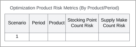
The stocking point count and supply make count risks are aggregations across every product and period. The individual risk scores can be found in the ProductRiskMetrics tables.
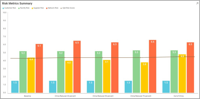
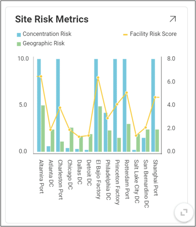
We can use our visualization tools to get a better sense of how risk varies across design scenarios.
With Optilogic’s new Teams feature set (see the "Getting Started with Optilogic Teams" help center article) working collaboratively on Cosmic Frog models has never been easier: all members of a team have access to all contents added to that team’s workspace. Centralizing data using Teams ensures there is a single source of truth for files/models which prevents version conflicts. It also enables real-time collaboration where files/models are seamlessly shared across all team members, and updates to any files/models are instantaneous for all team members.
However, whether your organization uses Teams or not, there can be a need to share Cosmic Frog models, for example to:
In this documentation we will cover how to share models, and the different options for sharing. Sharing models can be from an individual user or a team to an individual user or a team. As the risk of something undesirable happening with the model when multiple people work on it increases, it is important to be able to go back to a previous version of the model. Therefore, it is best practice to make a backup of a model prior to sharing it. Continue making backups when important/major changes are going to be made or when wanting to try out something new. How to make a backup of a model will be explained in this documentation too and will be covered first.
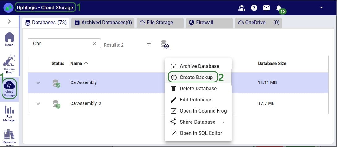
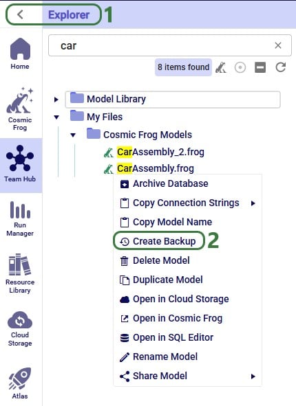
A backup of a model is a snapshot of its exact state at a certain point in time. Once a backup has been made, users can use them to revert to if needed. Initiating the creation of a backup of a Cosmic Frog model can be done from 3 locations within the Optilogic platform: 1) from the Models module within Cosmic Frog, 2) through the Explorer and 3) from within the Cloud Storage application on the Optilogic platform. The option from within Cosmic Frog will be covered first:
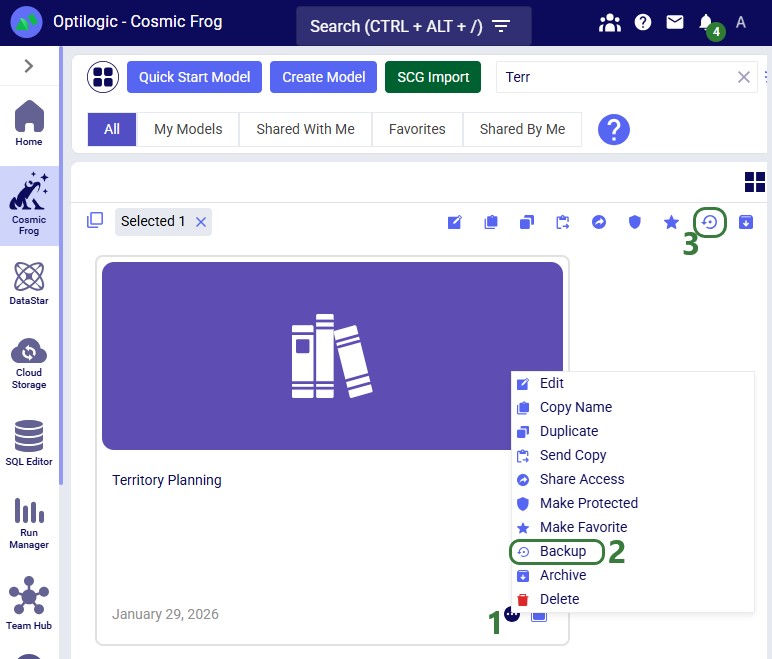
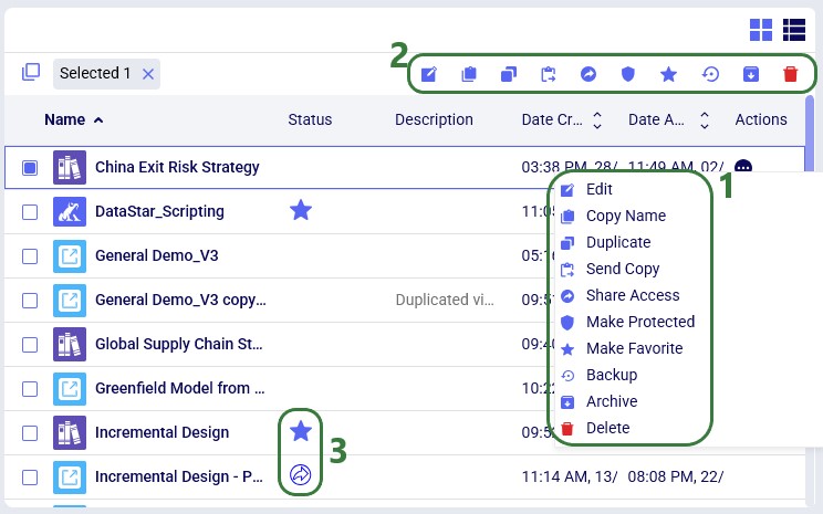
When in the Models module of Cosmic Frog (aka the Model Manager), hover over the model you want to create a backup for, and click on the icon with 3 horizontal dots that comes up at the bottom right of the model card (1). This brings up the model management options context menu, from which you can choose the Backup option (2). If only 1 model is selected, the Backup option can also be accessed from the toolbar at the top of the model list/grid (3).
From the Cloud Storage application it works as follows:
Through the Explorer, the process is similar:
Whether from the Models module within Cosmic Frog, through the Cloud Storage application or via the Explorer, in all 3 cases the Create Backup form comes up:
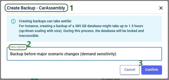
After clicking on Confirm, a notification at the top of the user’s screen will pop up saying that the creation of a backup has been started:

At the same time, a locked database icon with hover over text of “Backup in progress…” appears in the Status field of the model database (this is in the Cloud Storage application’s list of databases):

This locked database icon will disappear again once the backup is complete.
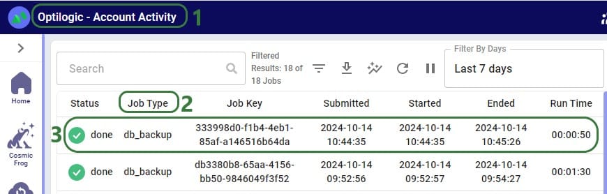
Users can check progress of the backup by going to the user’s Account menu under their username at the right top of the screen and selecting “Account Activity” from the drop-down menu:
To access any backups, users can expand individual model databases in the Cloud Storage application:

There are 2 more columns in the list of databases that are not shown in the screenshot above:

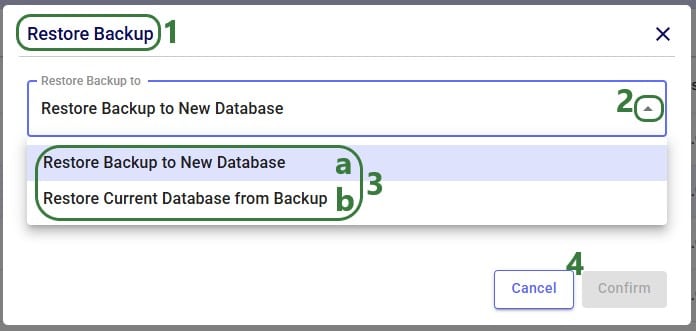
When choosing to restore a backup, the following form comes up:
Now that we have discussed how models can be backed up, we will cover how models can be shared. Note that it is best practice to make a backup of your model before sharing it.
If your organization uses Teams, first make sure you are in the correct workspace, either a Team’s or your personal My Account area, from which you want to share a model. You can switch between workspaces using the Team Hub application, which is explained in this "Optilogic Teams - User Guide" help center article.
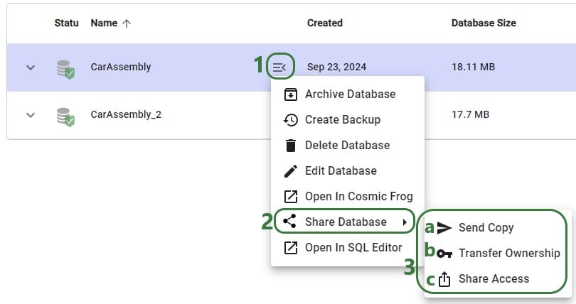
Like making a backup of a model database, sharing a model can also be done through the Cloud Storage application and the Explorer. Starting with the Cloud Storage option:
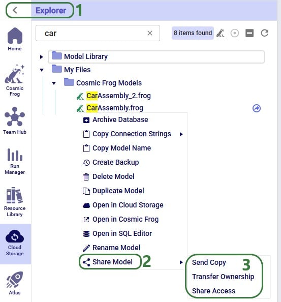
The Share Model options can also be accessed through the Explorer:
Now we will cover the steps of sending a copy of a model to another user or team. The original and the copy are not connected to each other after the model was shared in this way: updates to one are not reflected in the other and vice versa.

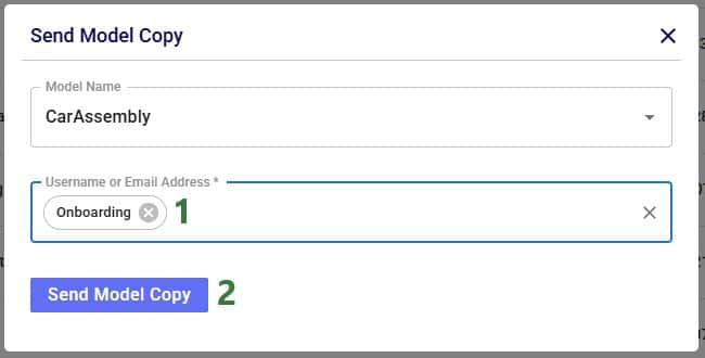
After clicking on the Send Model Copy button, a message that says “Model Copy Sent Successfully” will be displayed in the Send Model Copy form. Users can go ahead and send copies of other models to other user(s)/teams(s) or close out of the form by clicking on the cross icon at the right top of the form.
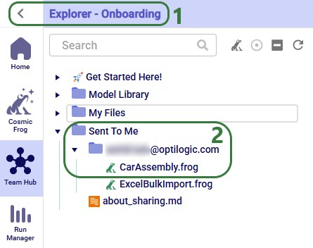
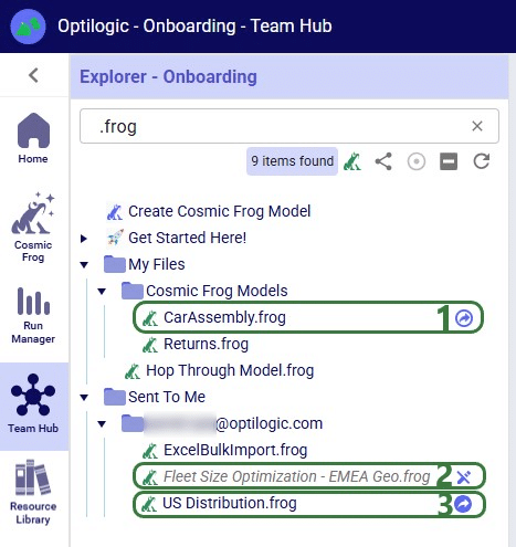
In this example, a copy of the CarAssembly model was sent to the Onboarding team. In the Onboarding team’s workspace this model will then appear in the Explorer:
Next, we will step through transferring ownership of a model to another user or team. The original owner will no longer have access to the model after transferring ownership. In the example here, the Onboarding team will transfer ownership of the Tariffs model to an individual user.
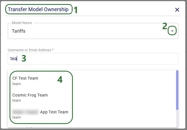
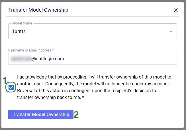
After clicking on the Transfer Model Ownership button, a message that says “Transferred Ownership Successfully” will be displayed in the Transfer Model Ownership form. Users can go ahead and transfer ownership of other models to other user(s)/teams(s) or close out of the form by clicking on the cross icon at the right top of the form.
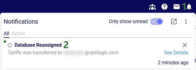
There will be a notification of the model ownership transfer in the workspace of the user/team that performed the transfer:
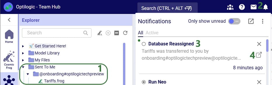
The model now becomes visible in the My Account workspace of the individual user the ownership of the model was transferred to:
Lastly, we will show the steps of sharing access to a model with a user or team. Note that Sharing Access to a model can be done from Explorer and from the Cloud Storage application (same as for the Send Copy and Transfer Ownership options), but can also be done from the Models module in Cosmic Frog:
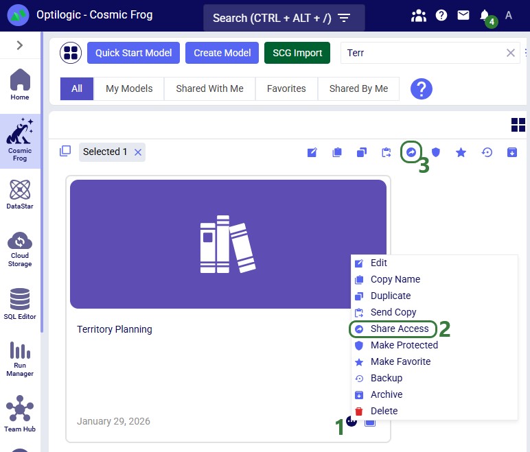
In Cosmic Frog's Models module (aka Model Manager), hover over the model card of the model you wan to share access to and then click on the icon with 3 horizontal dots that comes up in the bottom right of the model card (1). Clicking on this icon brings up the model management actions context menu, from which you can choose the Share Access option (2). If only 1 model is selected, the Share Access option is also available from the model management actions toolbar at the top of the model list/grid (3).
In our walk-through example, an individual user will share access to a model called "Fleet Size Optimization - EMEA Geo" with the Onboarding team.
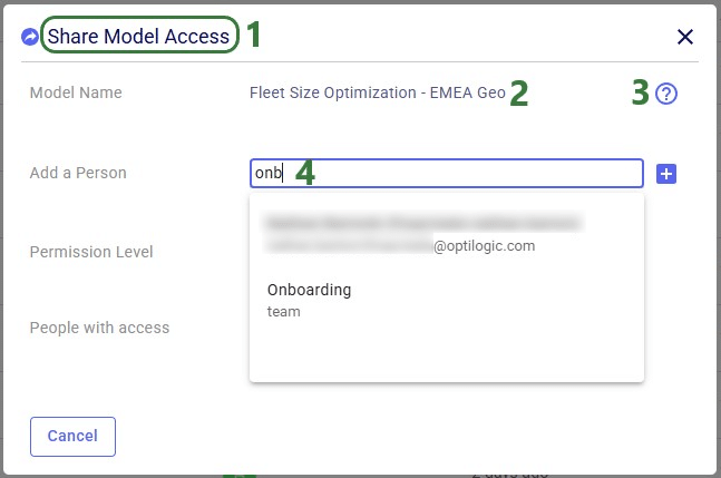
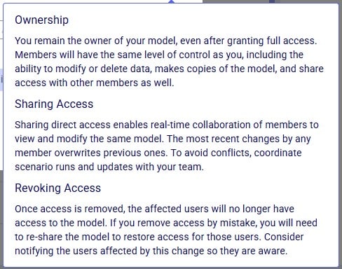
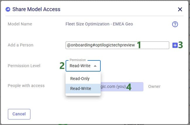
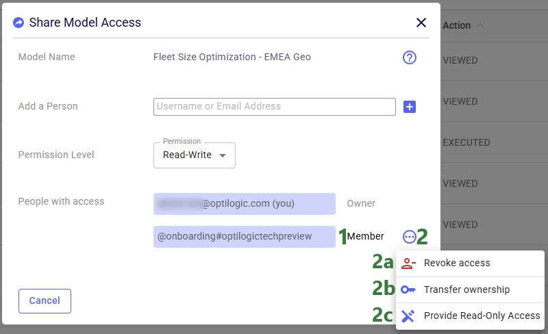
After the plus button was clicked to share access of the Fleet Size Optimization - EMEA Geo model with the Onboarding team, this team is now listed in the People with access list:
Now, in the Onboarding team’s workspace, we can access this model, of which the team receives a notification too:
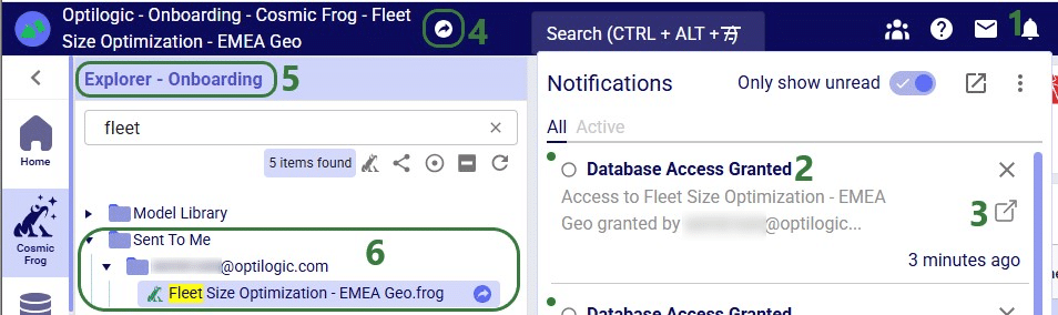
Now that the Onboarding team has access to this model, they can share it with other users/teams too: they can either send a copy of it or share access, but they cannot transfer ownership as they are not the model’s owner.
In the Explorer of the workspace of the user/team who shared access to the model, a similar round icon with arrow inside it will be shown next to the model’s name. The icon colors are just inverted (blue arrow in white circle) and here the hover text is “You have shared this database”, see the screenshot below. There will also be a notification about having granted access to this model and to whom (not shown in the screenshot):

If the model owner decides to revoke access or change the permission level to a shared model, they need to open the Share Model Access form again by choosing Share Access from the Share Model options / clicking on the Share icon when hovering over the model's card on the Cosmic Frog start page:
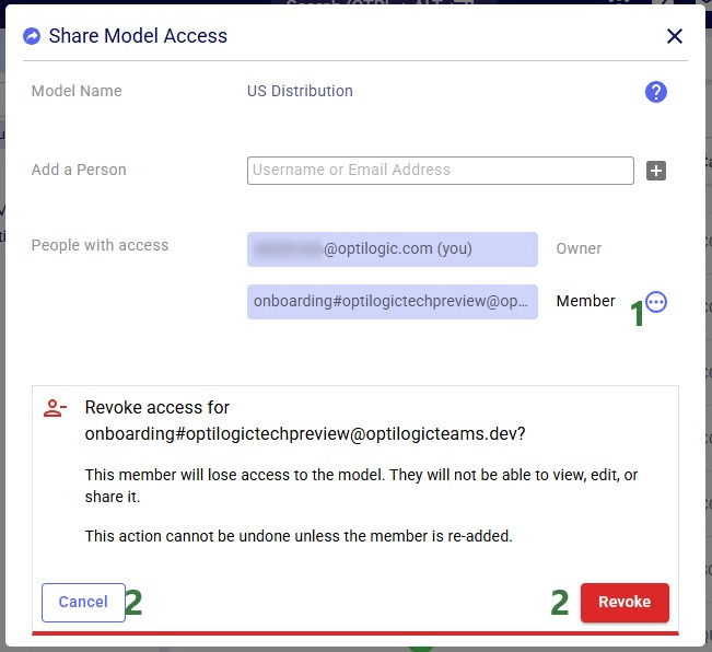
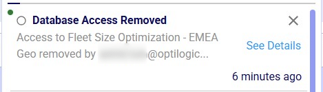
If access to a model is revoked, the team/user that was previously granted access but now no longer will have access, receives a notification about this:
With Read-Only access, teammates and stakeholders can explore a shared model, view maps, dashboards, and analytics, and provide feedback — all while ensuring that the data remains unchanged and secure.
Read-Only mode is best suited for situations where protecting data integrity is a priority, for example:
See the Appendix for a complete list of actions and whether they are allowed in Read-Only Access mode or not.
Similar to revoking access to a previously shared model, in order to change the permission level of a shared model, user opens the Share Model Access form again by choosing Share Access from the Share Model options / clicking on the Share icon when hovering over the model's card on the Cosmic Frog start page:
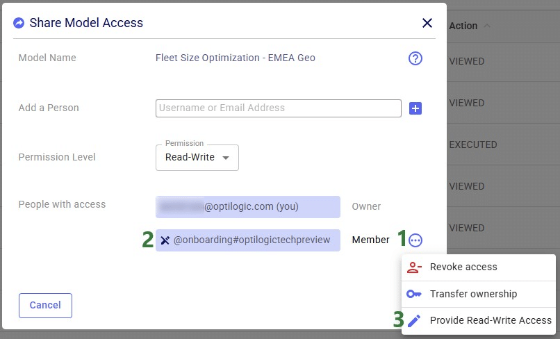
Models with Read-Only access can be recognized on the Optilogic platform as follows:
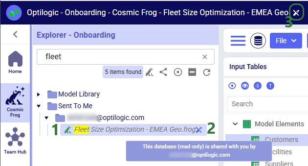
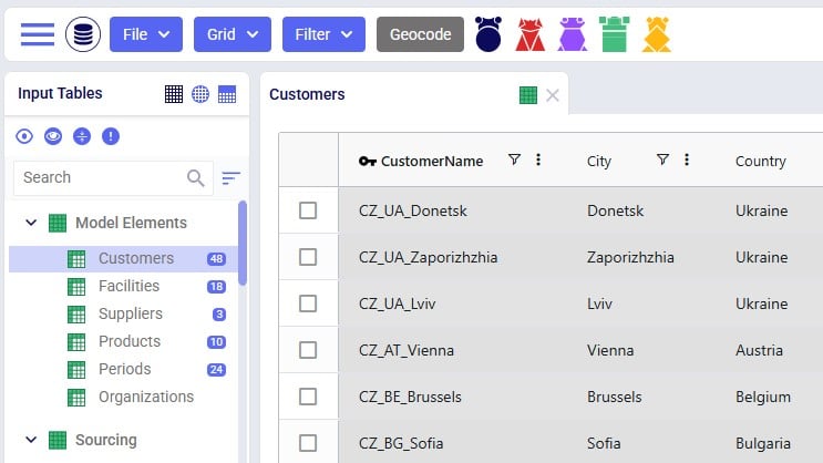
Input tables of Read-Only Cosmic Frog models are greyed out (like output tables already are by default), and and write actions (insert, delete, modify) are disabled:
Read-Only models can be recognized as follows in other Optilogic applications:
When working with models that have shared access, please keep following in mind:
In addition to the various ways model files can be shared between users, there is a way to share a copy of all contents of a folder with another user/team too:
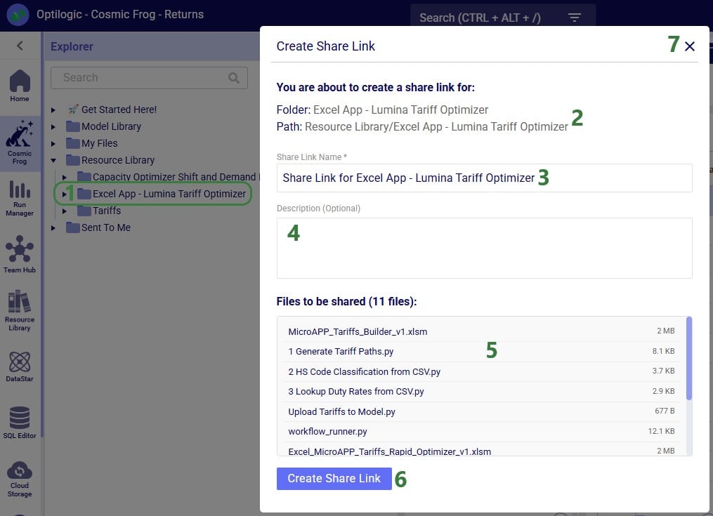
After clicking on the Create Share Link button, the share link is copied to the clipboard. A toast notification of this is temporarily displayed at the right top in the Optilogic platform. The user can paste the link and send it to the user(s) they want to share the contents of the folder with.
When a user who has received the share link copies it into their browser while logged into the Optilogic platform, the following form will be opened:
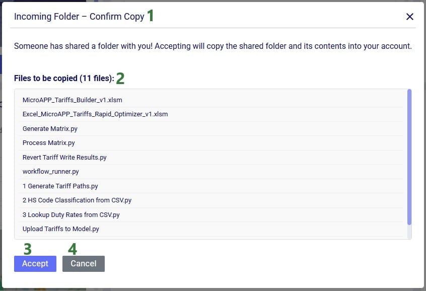
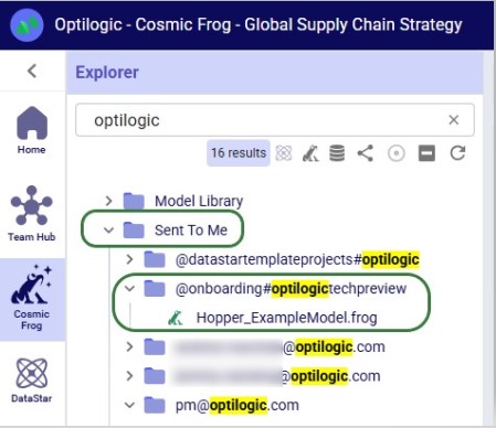
Folders copied using the share link option will be copied into a subfolder of the Sent To Me folder. The name of this subfolder will be the username / email of the user / team that sent the share link. The file structure of the sent folder will be maintained and appear the same as it was in the account of the sender of the share link.
See the View Share Links section in the Getting Started with the Explorer help center article on how to manage your share links.
Action - Allowed? - Notes:
The Model Manager in Cosmic Frog is the central place to create, view, organize, and maintain your supply chain models. It provides tools for quickly finding models, understanding their status, and performing common management actions such as editing, duplicating, and deleting models.
This guide walks you through the Model Manager interface step by step, explaining each major feature and control as it appears on screen. Screenshots are annotated with green outlines to highlight key areas, and numbered callouts are explained in corresponding lists so you can easily follow along.
When logged into the Optilogic platform, you can open Cosmic Frog by clicking on its icon in the list of applications on the left. Note that the order of the applications may be different in your list so you may need to scroll down:
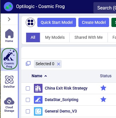
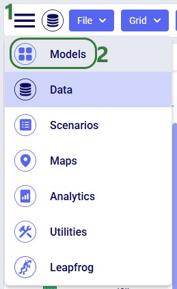
After opening Cosmic Frog, the model manager will typically be the active module. However, if you have been working in a specific model in Cosmic Frog previously, it may immediately open that model with its Data module being the active module. In that case, you can open the Model Manager from within Cosmic Frog by clicking on the icon with 3 horizontal bars at the left top to open the Module Menu, then select Models:
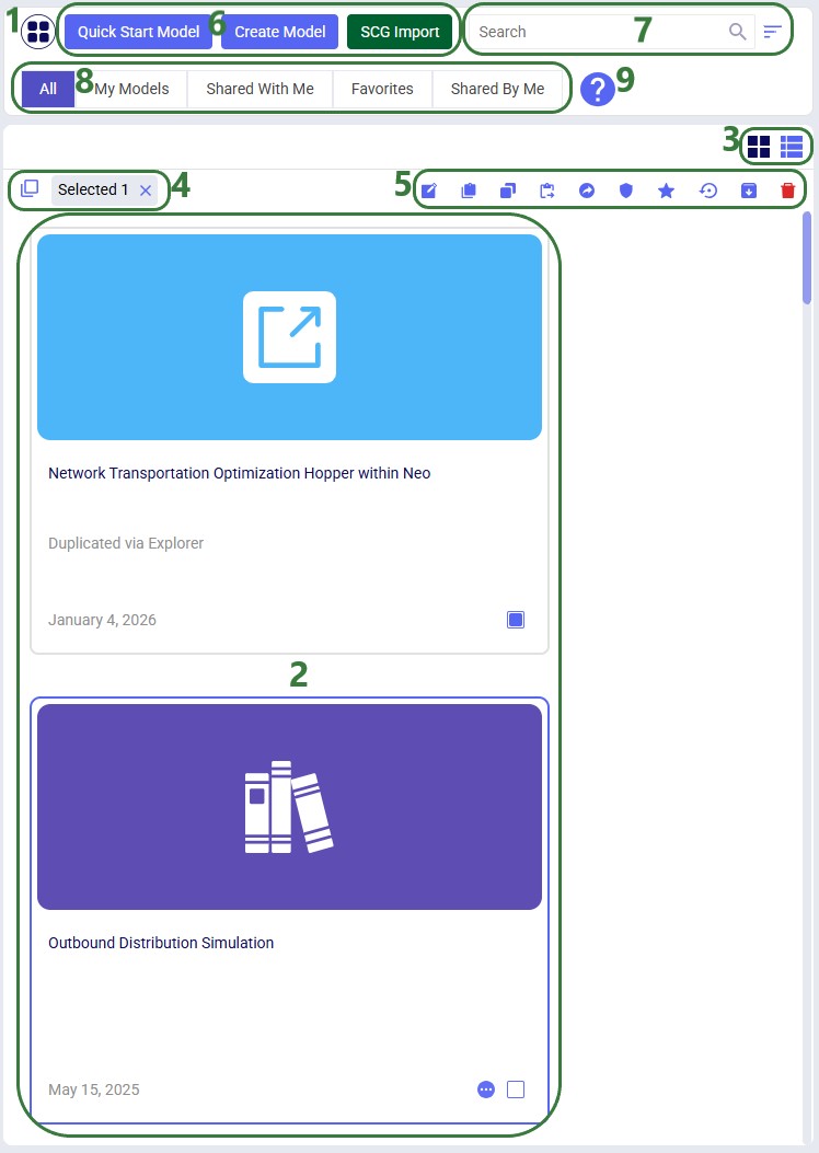
The Model Manager screen displays a table or grid of your existing models along with high level details such as name, status, and last modified date. This view is designed to give you immediate insight into your model library. The following screenshot shows at a high level the different features of the model manager. Each feature will be explained in more detail in subsequent sections of this documentation:
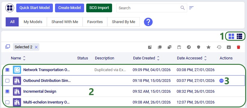
In the following screenshot we have switched from card view to list view:
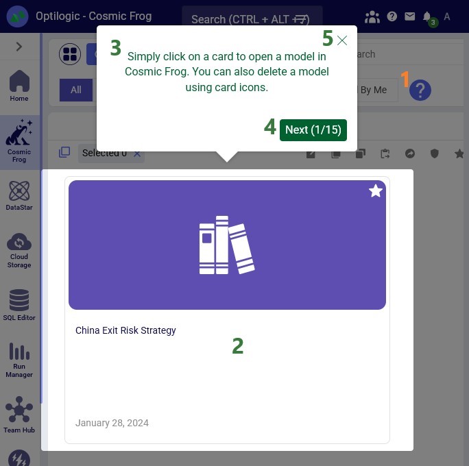
The Help & Hints area provides contextual guidance to help users understand the purpose of the Model Manager and how to use it effectively. These hints are especially useful for new users:
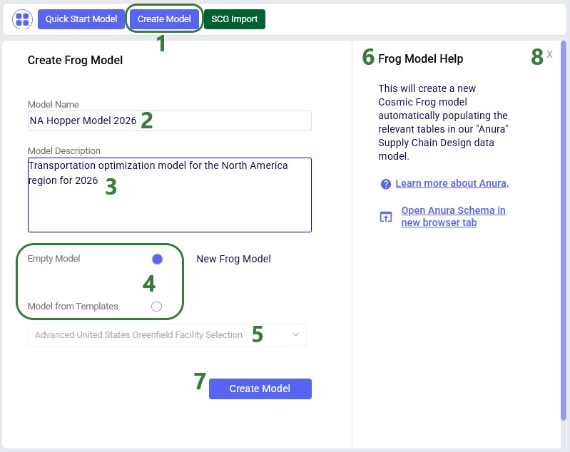
From the Model Manager there are a few options to create a new Cosmic Frog model, which will be covered in this section. We will start with the option from which new empty models as well as copies from Resource Library models can be created:
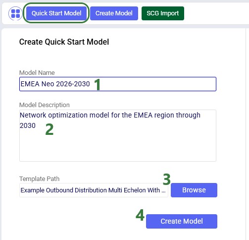
Another option to create a new model is to create one with tables populated from an Excel template, click on the Quick Start Model button to open the Create Quick Start Model form:
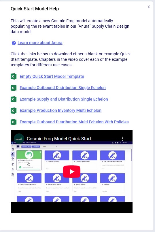
Note that for this option there is help available on the right-hand side of the form too, including example Excel template files, which can be downloaded to function as a starting point to overwrite with your own data. A video on this Quick Start option can be accessed from here too:
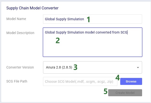
Finally, users also have the option to convert their Supply Chain Guru (SCG) models to a Cosmic Frog model. After clicking on the SCG Import button, the following Supply Chain Model Converter form comes up:
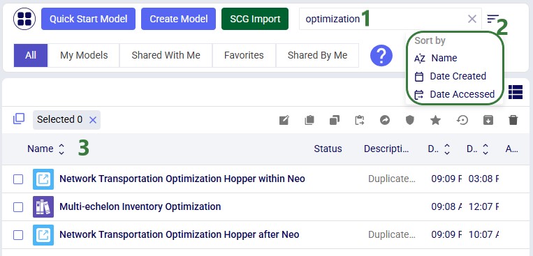
As your model library grows, search, sort, and filter tools help you quickly locate the models you need. The following screenshot shows the use of the search box and the available sort options:
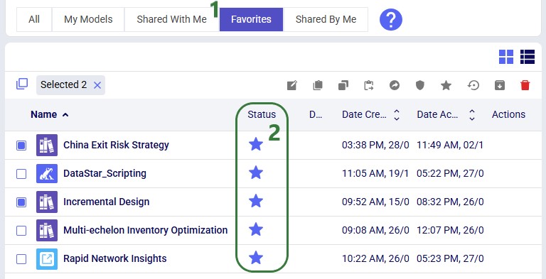
Standard filters to reduce the list of models to those of interest are also available:
To learn more about sharing models, please see this "Model Sharing & Backups for Multi-User Collaboration in Cosmic Frog" help center article.
The Model Manager provides comprehensive model management capabilities through both the action toolbar and context menus. The first 2 screenshots in this section show these in card view, while the last screenshot shows the options while in list view:
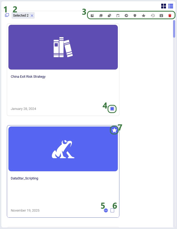
The model management actions available from the toolbar and from the context menu of a model in card view are shown in this next screenshot:
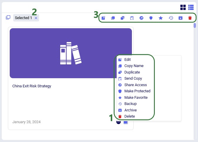
Lastly, the next screenshot shows the Model Management Actions while in list view:
Exciting new features which enable users to solve both network and transportation optimization in one solve have been added to Cosmic Frog. By optimizing multi-stop route optimization as part of Network Optimization, it enables users to streamline their analysis and make their Network Optimization more accurate. This is possible because the single optimization solve calculates multi-stop route costs by shipment/customer combination, uses this cost as part of another possible transportation mode in addition to OTR, Rail, Air, etc. and will result in more accurate answers by including better transportation costs in a single solve.
In addition to this documentation, these 2 videos cover the new Network Transportation Optimization (NTO) features too:
Network Transportation Optimization is particularly useful for two classic network design problems (both will be described in more detail in the next section):
This feature set includes 2 ways of running the Transportation Optimization (Hopper) and Network Optimization (Neo) engines together:
Following will be covered in this documentation for both the Hopper within Neo and Hopper after Neo NTO algorithms: example use cases, model inputs, how to use the new features, basics of the model used to show the NTO features, and walk through 2 example models, including their setup (input tables, scenarios), and analysis of the outputs using tables and maps.
With this feature, users can consider routes as inputs in a Neo model, meaning that the model will optimize product flow sources based on all costs, including the cost of routes. Costs and asset capacities are taken into account for the routes.
Two example use cases which can be addressed using Hopper within Neo are customer consolidation and hub optimization, which will be illustrated with the images that follow.
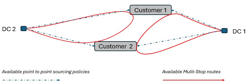
Consider a network where 2 distribution centers (DCs) are available to serve the customers. Two of these customers are in between the DCs and can either be serviced by the DCs directly (the blue dashed point to point lines) or product can be delivered to both of them as part of a multi-stop route from either DC (the red solid lines):
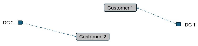
Running Neo without Hopper, not taking any route inputs into account, can lead to a solution where each DC serves 1 customer:
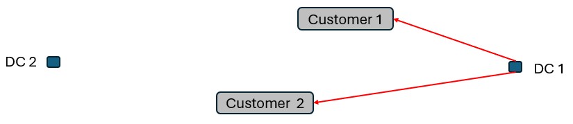
Whereas when taking route costs and capacities into account during a Hopper within Neo solve, it may be found that the overall cost solution is lower if one of the DCs (DC 1 in this example) serves both customers using a multi-stop route:
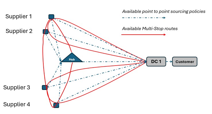
As a second example, consider a network where Suppliers can either deliver product to a Hub, either direct or on a multi-stop route from multiple suppliers, or direct/on multi-stop routes from multiple suppliers to a Distribution Center. Again, blue dashed lines indicate direct point to point deliveries and red lines indicate multi-stop route options:
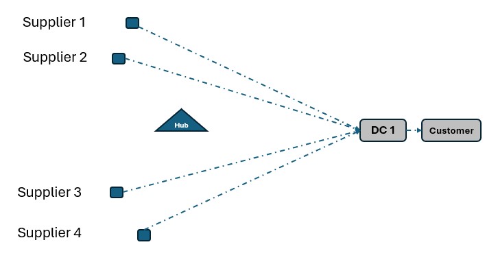
Not taking route options into account when running Neo without Hopper can lead to a solution where each Supplier delivers to DC 1 directly:
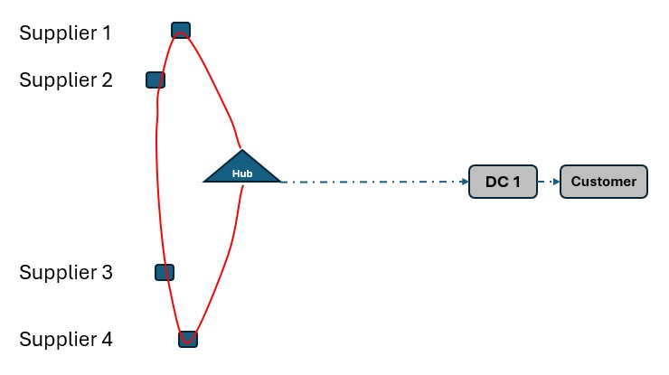
This solution can change to one where the Suppliers deliver to the Hub on a multi-stop route when taking the route options into account in a Neo within Hopper run if this is overall beneficial (e.g. lower total cost) to do:
The Hopper within Neo algorithm needs inputs in order to consider routes as part of the Neo network optimization run. These include:
In all cases, additional records need to be added to the Transportation Policies table as well (explained in more detail below), and if the Transit Matrix table is populated, it will also be used for Hopper within Neo runs.
Please note that any other Hopper related tables (e.g. relationship constraints, business hours, transportation stop rates, etc.), whether populated or not, are not used during a Hopper within Neo solve.
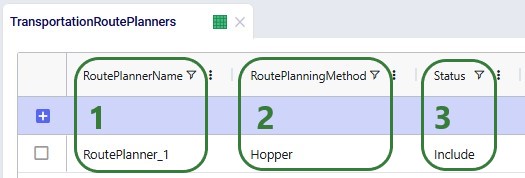
To use the Hopper algorithm for route generation, the Transportation Route Planners table and Transportation Policies tables need to be used. Starting with the Transportation Route Planners table:
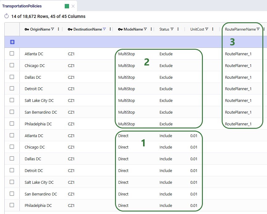
In the Transportation Policies table, records need to be added to indicate which lanes will be considered to be part of a multi-stop route:
Under the hood, potential routes will be calculated based on the inputs provided by the user. For example, for a case where the shipments table is not populated, and the user has specified their own assets:
As a numbers example to illustrate this calculation of a candidate route, let us consider following:
These costs are then used as inputs into the Network Optimization, together with costs for other transportation modes, and all are taken into account when optimizing the model.
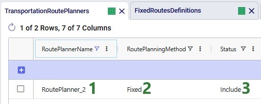
To use routes that are defined by the user in the Neo solve, the user also needs to use the Transportation Route Planners table, in combination with the Fixed Routes, Fixed Routes Definitions, and Transportation Policies tables. Starting with the Transportation Route Planners table:
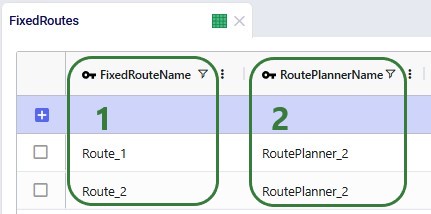
The Fixed Routes table connects the names of the routes the user defines with the route planner name:
There are a few additional columns on the Fixed Routes table which are not shown in the screenshot above. These are:
The Fixed Routes Definitions table needs to be used to indicate which stops are on a route together:
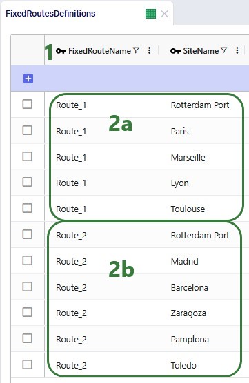
Please note that the Stop Number field on this table is currently not used by the Hopper within Neo functionality. The solve will determine the sequence of the stops.
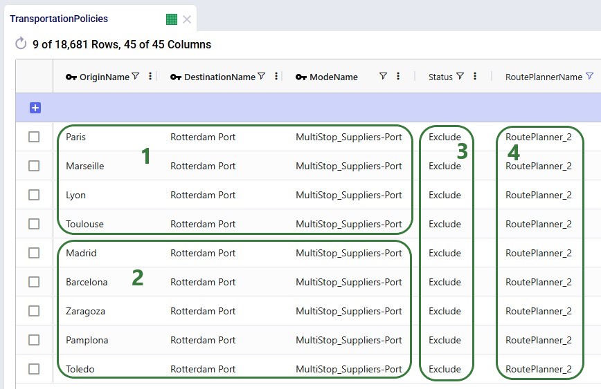
Finally, to understand which locations function as sources (pickups) and which as drop-offs (deliveries) on a route, and to indicate that multi-stop routes are an option for these source-destination combinations, corresponding records need to be added to the transportation policies table too:
A copy of the Global Supply Chain Strategy model from the Resource Library was used as the starting point for both the Hopper within Neo and Hopper after Neo demo models. The original Global Supply Chain Strategy model can be found here on the Resource Library, and a video describing it can be found in this "Global Supply Chain Strategy Demo Model Review" Help Center article. The modified models showing the Hopper within and after Neo functionality can be found here on the Resource Library:
To learn more about the Resource Library and how to use it, please see the "How to use the Resource Library" Help Center article.
A short description of the main elements in this model is as follows:
We illustrate the locations and flow of product through the following 3 maps:
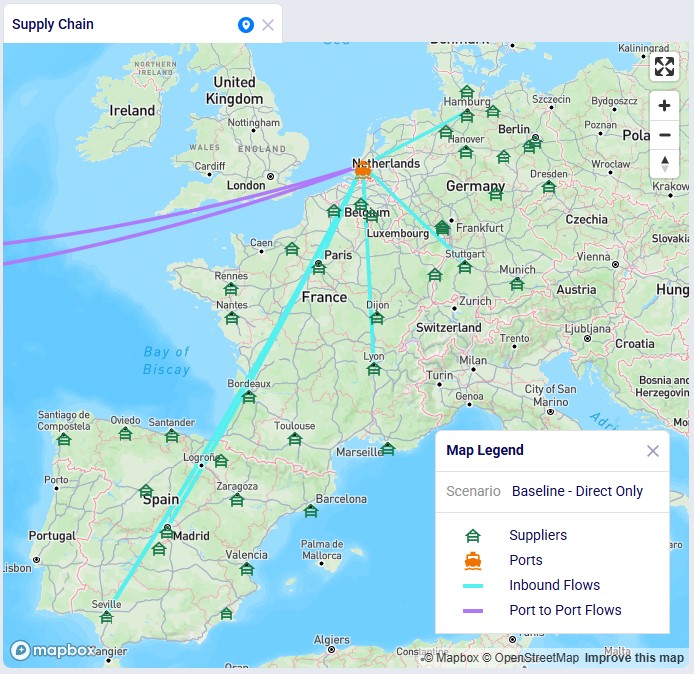
Even though around 35 suppliers are set up in the model in the EMEA region, only 6 of them are used based on the records in the Supplier Capabilities input table. We see the light blue lines from these suppliers delivering raw materials to the port in Rotterdam. From there, the 2 purple lines indicate the transport of the raw materials from Rotterdam to the US and Mexican ports.
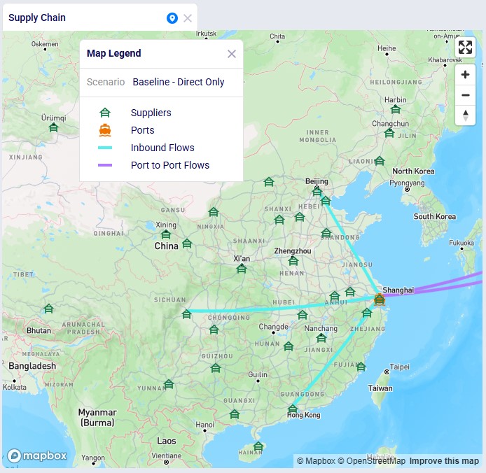
Similarly, around 35 suppliers are set up in China in the model, but only 3 of them are used per the set up in the Supplier Capabilities input table. The light blue lines are the transport of raw materials from the suppliers to the Shanghai port and the purple lines from the Shanghai port to the ports in Mexico and the US.
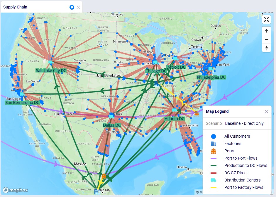
This map shows the flows into and within/between the US and Mexico locations:
We will show how Hopper routes for the last leg of the network, from DCs to customers, can be taken into account during a Neo solve. Through a series of scenarios, we will explore if using multi-stop routes for this supply chain is beneficial:
After copying the Global Supply Chain Strategy model from the Resource Library, following changes/additions were made to be able to consider Hopper generated routes for the DC-CZ leg during the Neo solve. After listing these changes here, we will explain each in more detail through screenshots further below. Users can copy this modified model with the scenarios, outputs, and preconfigured maps from the Resource Library.
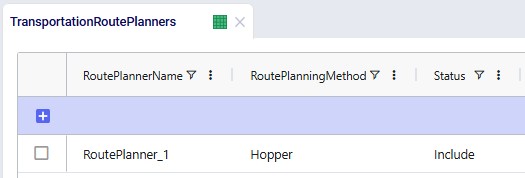
One record is added in this table where it is indicated that the route planner named "RoutePlanner_1" will use Hopper generated routes and is by default included during a Neo solve.
We choose to add our own asset instead of the 3 defaults ones that will be used if the Transportation Assets table is left blank. The characteristics of our large vehicle are shown in the next 2 screenshots:
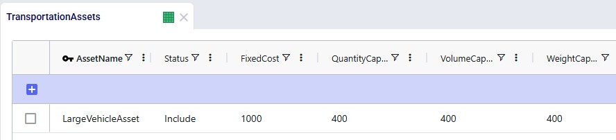
This large asset is included in the scenario runs as its Status = Include. The fixed cost of the asset is $1,000, with a capacity of 400 units / 400 cubic feet / 400 pounds.
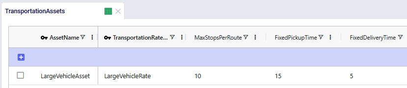
A rate record is set up in the Transportation Rates input table in order to model distance- and time-based costs. This is shown in the next screenshot. To use it, we link it to the asset by using the Transportation Rate Name field on the Transportation Assets table.
The Max Stops Per Route is set to 10. A Fixed Pickup Time of 15 minutes is entered, which will be applied once when picking up product at the DCs. Also, a Fixed Delivery Time of 5 minutes is set, this will be applied once at each customer when delivering product (the UOM fields are omitted in the screenshot; they are set to MIN).
Besides the fixed cost for the asset as specified in the Transportation Assets table, we also want to apply both distance- and time-based costs to the routes:
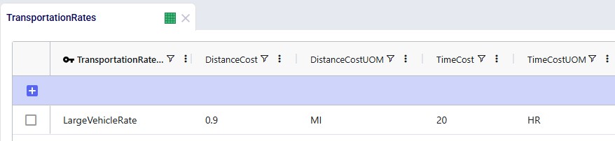
A record is set up in the Transportation Rates table where Transportation Rate Name is used in the Transportation Assets table to link the correct rate to the correct asset (e.g. LargeVehicleRate is used for the LargeVehicleAsset). The per distance cost is set to 0.9 per mile, and the time cost is set to 20 per hour; the latter mostly reflects the cost for the driver.
For the scenarios to use actual road distances and transport times, the Distance Lookup Utility in Cosmic Frog was used with following parameters:
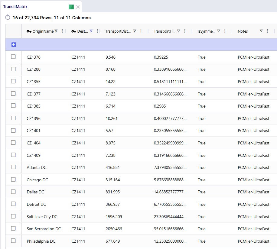
A subset of records filtered for 1 customer destination (CZ1411) is shown in this next screenshot where we see the distance and time from the 10 closest other customers to this customer, and also from all 7 DCs:
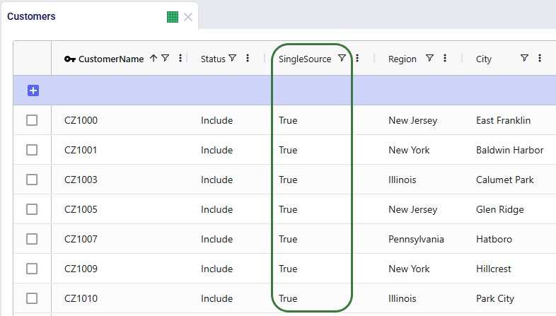
To remove potential dual sourcing, all customers are set to single sourcing (Single Source field is set to True on the Customers table), meaning they need to be served all product they demand from a single DC. In this model, setting customers to single sourcing also helps reduce the runtime of the scenarios:
To further help reduce solve times, a flow count constraint that allows the selection of at maximum 1 mode to each customer is added:
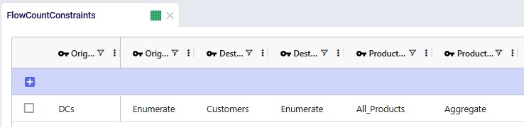
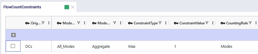
Groups for all DCs, all Customers, all Products, and all Modes (the 2 to customers, Direct and MultiStop) are being used in the Origin, Destination, Product, and Mode fields on the Flow Count Constraints table. The Group Behavior fields for Origin and Destination are set to Enumerate, meaning that under the hood, this constraint is expanded out into individual constraints for each DC-Customer combination. On the other hand, the Group Behavior fields for Product and Mode are set to aggregate, meaning that the constraint applies to all products and modes together. The Counting Rule indicates the combination of entities that "is counted on", in this case the number of modes, which is not allowed to be more than 1 (Type = Max and Value = 1), i.e. there can only be 1 mode selected on each DC-customer lane.
The Status field of the Flow Count Constraint is set to Exclude (not shown in the screenshots above), and the constraint will be included in 2 of the scenarios by changing the status through a scenario item.
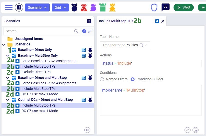
The following screenshot shows the scenarios and which scenario items are associated with each of them. To learn more about creating scenarios and their items, please see these 2 help center articles: "Creating Scenarios in Cosmic Frog" and "Getting Started with Scenarios".
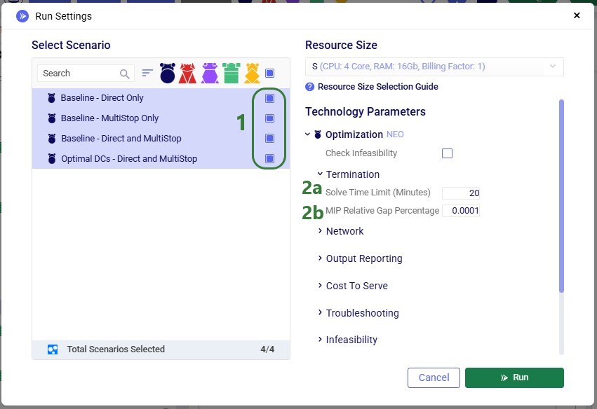
To find a balance between running the model to a low enough gap to reduce any suboptimality in the solution and running for a reasonable amount of time, the following is set on the Run Settings modal which comes up after clicking on the green Run button at the top right in Cosmic Frog:
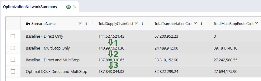
We will first look at the Optimization Network Summary and Optimization Flow Summary output tables, and next at the maps of the last 2 scenarios. We will start with the Optimization Network Summary output table. This screenshot does not show the Production and Fixed Operating Costs as they are the same across all scenarios, and we will focus on the transportation related costs:
Next, the Optimization Flow Summary output table is filtered for 1 specific customer, CZ215, for which the DC assignment is changed in the final scenario. The table is also filtered for the Rockets product, for which the delivered quantity is the same for these 4 records (1,243 units):
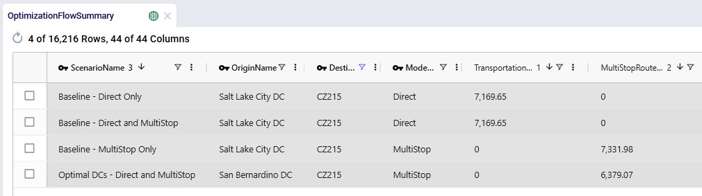
Salt Lake City is the optimal DC to source from for this customer based on just the direct delivery option; the transportation cost is ~7.2k. We see from the "Baseline - MultiStop Only" scenario that using a multi-stop route from Salt Lake City to this customer is a little more expensive (7.3k), so therefore the Direct mode is used in the "Baseline - Direct and MultiStop" scenario. In the "Optimal DCs - Direct and MultiStop" scenario, the customer swaps DC and is served using a multi-stop route from the San Bernardino DC, this results in a transportation cost of 6.4k, which is a reduction of almost $800 as compared to going direct from the Salt Lake City DC.
With a newly added output table named Optimization Flow Route Summary, we can see on which route from San Bernardino CZ215 is placed in this "Optimal" scenario:
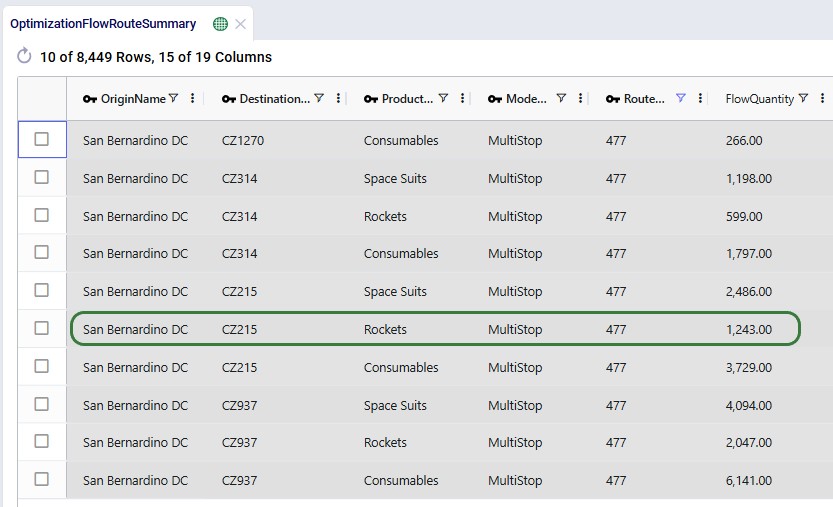
We see that CZ215 is a stop on route 477 from San Bernardino. The screenshot also shows the other stops on this route. Now we will retrace how the multi-stop route cost of $6.4k for this flow (see previous screenshot) is calculated:
When the possible routes are created during the model run, each customer is placed on up to 3 potential routes from its closest 2 DCs. These possible routes generated during preprocessing are listed in the HopperRouteSummary.csv input file which is generated when the "Write Input Solver" model run option (Troubleshooting section) is turned on. We can look up route 477 in it to see the cost for it:

The following 2 maps show the DC-CZ flows for the "Baseline - Direct and MultiStop" and "Optimal DCs - Direct and MultiStop" scenarios. Multi-stop routes are shown with blue lines and direct deliveries with red lines. There are 15 customers that swap DCs and these are shown with larger red dots:
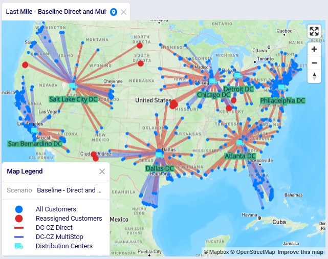
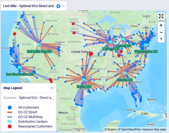
In total 15 CZs are swapping DCs in the "Optimal DCs - Direct and MultiStop" scenario. From west to east on the map:
The last 3 swaps cause some flow lines to be crossing each other on the map. This is due to the algorithm considering a finite number of possible routes.
Note that maps for the first 2 scenarios are also set up in this demo model.
Re-running these scenarios in future with a newer solver and/or after making (small) changes to the model can change the outputs such that the set of reassigned customers which are shown in larger red dots on the map changes. To visualize these on the map in the same way as is done above, the filter in the Condition Builder panel of the "Reassigned Customers" map layer needs to be updated manually. Currently the filter is as follows:
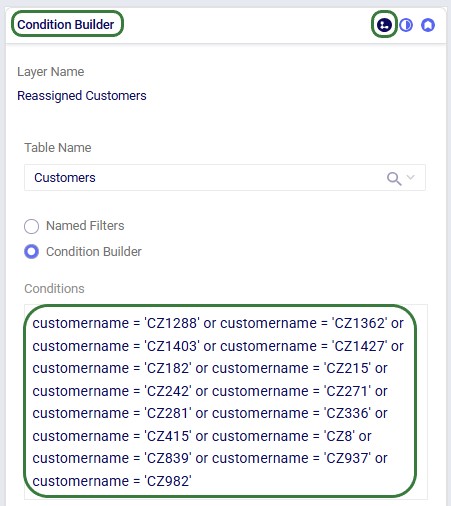
To determine which customers are being reassigned and need to be used in this filter, users can take following steps (which can be automated using for example DataStar):
With this new functionality, a transportation optimization (Hopper) run is started immediately after a network optimization (Neo) run has completed and this will be seen as one run to the user. Underneath, the assignments on the last leg of the network (e.g. customer to DC assignments) as determined optimal by the Neo run will be fixed for the Hopper run, and then multi-stop routes are generated for this last leg during the Hopper run. All existing Hopper functionality is taken into account while determining the optimal multi-stop routes and complete sets of outputs for both the network optimization and transportation optimization are generated at the end of a Hopper after Neo run. This saves users time where they do not need to go into the model to retrieve and manipulate Neo outputs to be used as input shipments for a subsequent Hopper run.
Besides needing the usual input for the network optimization (Neo) engine to be able to run, the Hopper after Neo algorithm needs some additional inputs in order to generate optimal multi-stop routes after the Neo run has completed. These include:
In addition, all populated Hopper fields used on any other Hopper table will be used during the Hopper part of the solve.
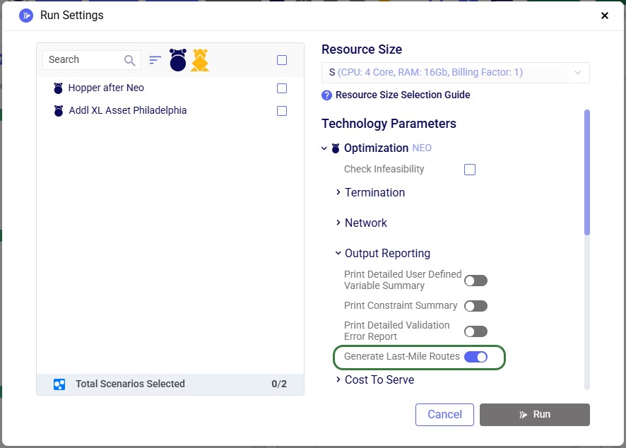
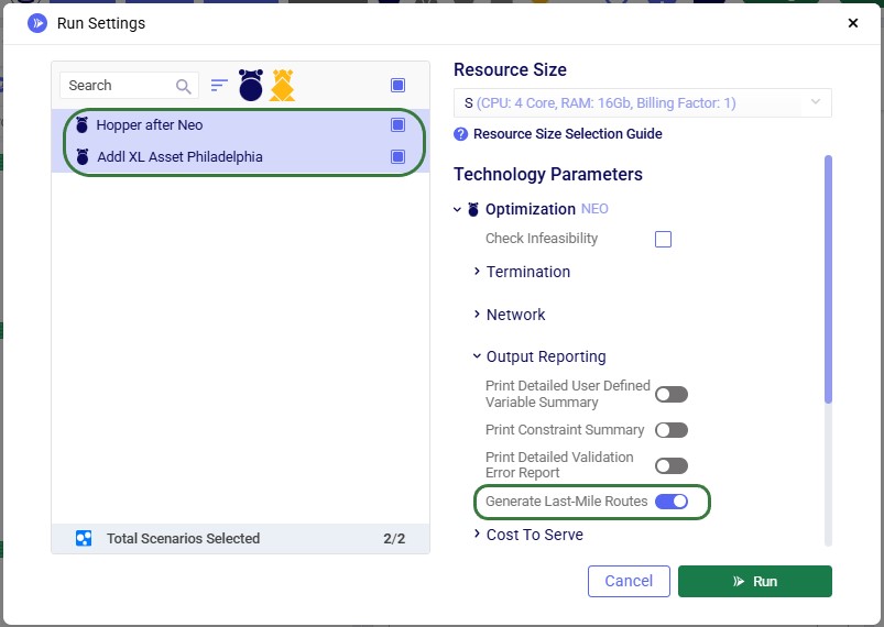
To turn on the Hopper after Neo functionality, one needs to enable the "Generate Last-Mile Routes" run setting in the Output Reporting section of the Optimization (NEO) Technology Parameters. These parameters are located on the right-hand side of the Run Settings modal which comes up after clicking on the green Run button at the right top in Cosmic Frog:
Please see the "Model used to showcase Hopper within/after Neo Features" section further above for the details of the starting point for the demo model for Hopper after Neo, which is the same one that was also the starting point for the Hopper within Neo demo model.
We will show how Hopper routes for the last leg of the network, from DCs to customers, can be created immediately after a Neo solve. Through 2 scenarios, we will explore which asset mix will be optimal for the generated multi-stop routes:
After copying the Global Supply Chain Strategy model from the Resource Library, following changes/additions were made to be able to use Hopper for multi-stop route generation for the DC-CZ leg after the Neo solve. After listing these changes here, we will explain each in more detail through screenshots further below. Users can copy this modified model with the scenarios and outputs from the Resource Library.
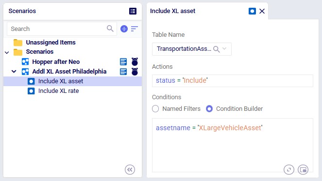
Instead of using the 1 large default vehicle when leaving the Transportation Assets table blank, we decide to use 2 user-defined assets initially: a large and medium one. One additional extra large asset will be added after running the first scenario with the 2 assets; it will be added to resolve unrouted shipments seen in the first scenario. The assets and their settings are shown in the following 2 screenshots:
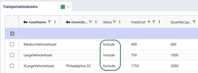
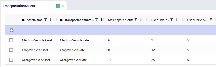
We see that both the Medium and Large vehicle are available at all locations (Domicile Location is left blank) and their Status is set to "include", whereas the Extra Large vehicle will only be available at the Philadelphia DC in the second scenario, and its initial Status is set to "Exclude". The assets have increasing fixed costs, quantity capacities, max number of stops per route, and fixed pickup times (in minutes) by increasing asset size. The fixed delivery time is the same for all: 5 minutes per stop.
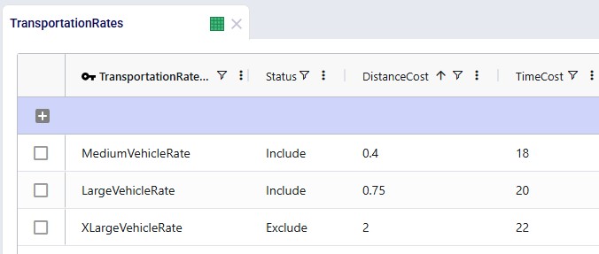
For each asset, a transportation rate is specified in the Transportation Rates input table. This rate is used in the Transportation Rate Name field in the Transportation Assets table (see screenshot above). The Distance and Time Costs are specified as follows, where the distance-based rate increases with the size of the vehicle to account for higher fuel usage. The Time Cost increases a bit with the size of the vehicle too to reflect the level of experience of the driver needed for larger vehicles:
Two scenarios will be run in this model:
When running the scenarios, the only additional input required to indicate that the Hopper engine should be run immediately after the Neo run, while taking its customer assignment decisions into account, is to turn on the "Generate Last-Mile Routes" option in the Output Reporting section of the Optimization Technology Parameters:
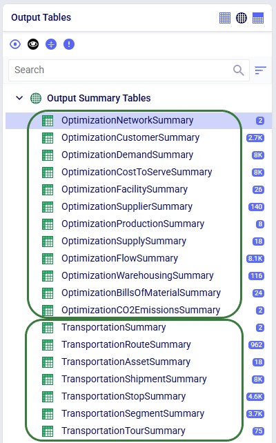
After running both scenarios, we see that full sets of outputs have been generated in the network optimization output tables and in the transportation optimization output tables:
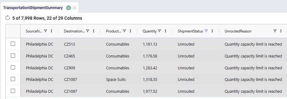
When looking through all outputs, we notice unrouted shipments in the Transportation Shipment Summary output table. Filtering these out, we find they are all shipments coming from Philadelphia DC, and the Unrouted Reason for all = "Quantity capacity limit is reached", see the next screenshot. The large vehicle asset has a capacity of 1000 units which is not big enough to fit these shipments. Therefore, the XL asset is added at Philadelphia DC in the second scenario.
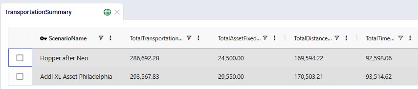
After running the second scenario, there are no more unrouted shipments and we take a look at the Transportation Summary output table which summarizes the Hopper part of the run at the scenario level. We can conclude from here that also delivering these 5 large shipments adds about $6.9k per week to the total transportation cost:
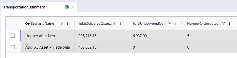
The following screenshot shows fields further to the right in the Transportation Summary output table, which confirm there are no more unrouted shipments in the second scenario, and therefore the total undelivered quantity is also 0 in this scenario:
Looking on a map, we can visualize the routes. In this example, they are colored based on which vehicle is used on the route. This is the map for the "Hopper after Neo" scenario. The map is called "Routes - Baseline" and is pre-configured when copying this model from the Resource Library:
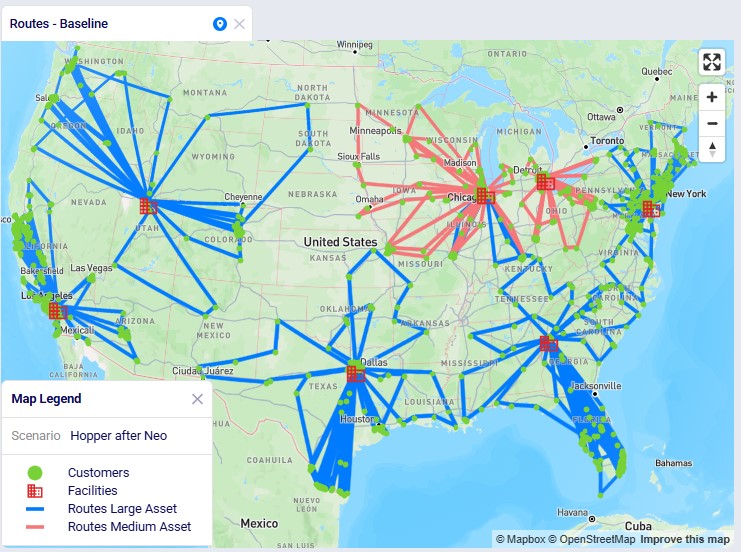
We see that the medium asset is used for most routes from the Chicago DC and all routes from the Detroit DC; the large asset is used on all other routes.
Finally, in the next screenshot we compare the 2 scenarios side-by-side, zoomed in on the Philadelphia DC and its routes. The darker routes are those that use the XL asset. Only the 10 customers which are served by the XL asset in the second scenario are shown on the map. Six of them were served by the large asset in the "Hopper after Neo" scenario; these are shown in orange on the map. The other 4 which are colored yellow had unrouted shipments for 1 or more products in the "Hopper after Neo" scenario; three of these are clustered together northeast of Philadelphia, while one is by itself southwest of Philadelphia:
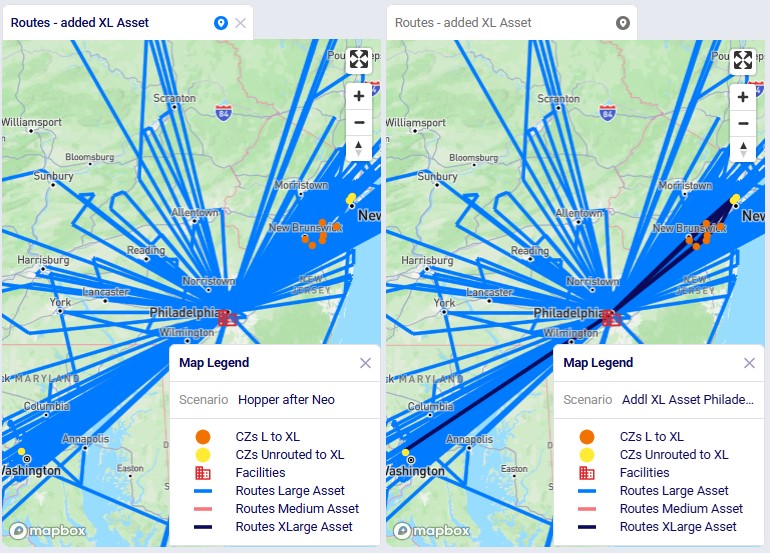
Please note that the "CZs L to XL" and "CZs Unrouted to XL" map layers contain filters on the Condition Builder pane that have been manually added after analyzing and comparing the outputs of the 2 scenarios to determine which customers to include in these layers. If the scenarios are re-run in future with a newer solver and/or after making (small) changes to the model, the outputs may change, including which customers switch from a large to extra-large vehicle and/or those going from being unrouted to using the extra-large vehicle. In that case the current condition builder filters will need to be updated to visualize those changes on the map. See the notes at the end of the "Hopper within Neo-Outputs" section which apply here in a similar way.
To determine which customers initially have unrouted shipments and are served by the extra-large vehicle in the second scenario:
To determine which customers are served by a different asset in the second scenario as compared to the first:
We hope this provides you with the guidance needed to start using the Hopper with Neo features yourself. In case of any questions, please do not hesitate to reach out to Optilogic's support team on support@optilogic.com.
Territory Planning is a new capability in the Transportation Optimization (Hopper) engine that automatically clusters customers into geographic regions - territories - and restricts routes and drivers to operate within those territory boundaries. This reduces operational complexity, improves route consistency, and enables delivery-promise logic for end consumers.
Territory Planning is available today in Cosmic Frog for all users and is powered by an enhanced high-precision Genetic Algorithm. Please note that all Hopper models, whether using the new Territory Planning features or not, can now be run using this high-precision mode.
This "How-To Tutorial: Territory Planning" video explains the new feature:
In this documentation we will first cover the benefits of Territory Planning, next explain how it works in Cosmic Frog, and then take you through an example model showcasing the new feature.
Traditional routing optimization focuses on building the most cost-efficient set of routes. In many real-world operations, however, drivers do not cross territories. A driver consistently serving the same neighborhoods knows the roads, customer patterns, and service requirements.
Key benefits include:
With the Territory Planning feature one new Hopper input table and two new Hopper output tables are introduced.
Territory Planning requires one new input table, Territory Planning Settings, while supporting all existing Hopper tables. This table defines the characteristics and constraints of the territories to be created during the Hopper solve, and can be found in the Functional Tables section: 1. Territory Type: A descriptive name for the territory configuration (e.g., "Large Territories", "Balanced Small Territories").
The universal compatibility with all other Hopper tables ensures you can add territory planning to any existing Hopper model without needing to restructure your data.
Territory Planning generates two new output tables, the Transportation Territory Planning Summary and the Transportation Territory Assignment Summary, in addition to all standard Hopper outputs. The Transportation Territory Planning Summary table provides one record per territory with aggregate KPIs:
This table is useful for:
The Transportation Territory Assignment Summary table shows the detailed assignment of each customer to a territory:
This table enables:
Besides the 2 new output tables, the following existing transportation output tables have new fields Territory Name and Territory Type added to them: Routes Map Layer, Transportation Asset Summary, Transportation Segment Summary, and Transportation Stop Summary. This facilitates filtering on territories in these tables to for example quickly see which assets are used in which territories.
Territory Planning uses Hopper's advanced genetic algorithm to simultaneously optimize multiple objectives:
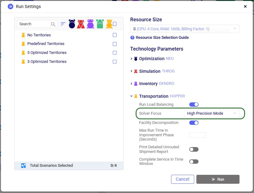
The genetic algorithm is available in Hopper's High Precision solver mode and powers all Hopper optimizations, not just territory planning. To turn on high precision mode, expand the Transportation (Hopper) section on the Run Settings modal which comes up after clicking on the green Run button at the right top in Cosmic Frog. Then select "High Precision mode" from the Solver Focus drop-down list:
A model showcasing the Territory Planning capabilities can be found here on Optilogic's Resource Library. We will cover its features, scenario configuration, and outputs here. You can copy this model to your own Optilogic account by selecting the resource and then using the Copy to Account blue button on the right hand-side (see this "How to use the Resource Library" help center article for more details).
First, we will look at the input tables of this model:
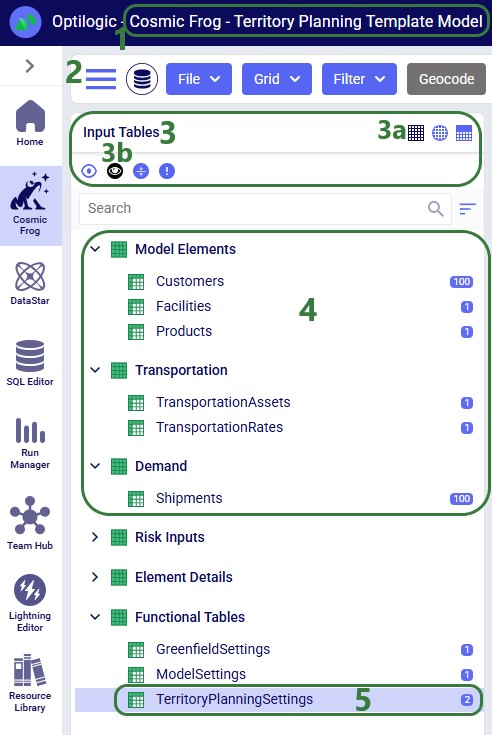
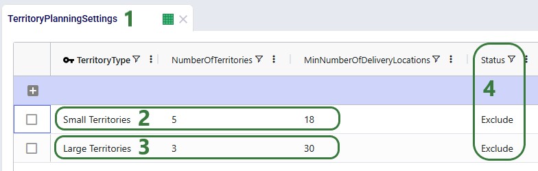
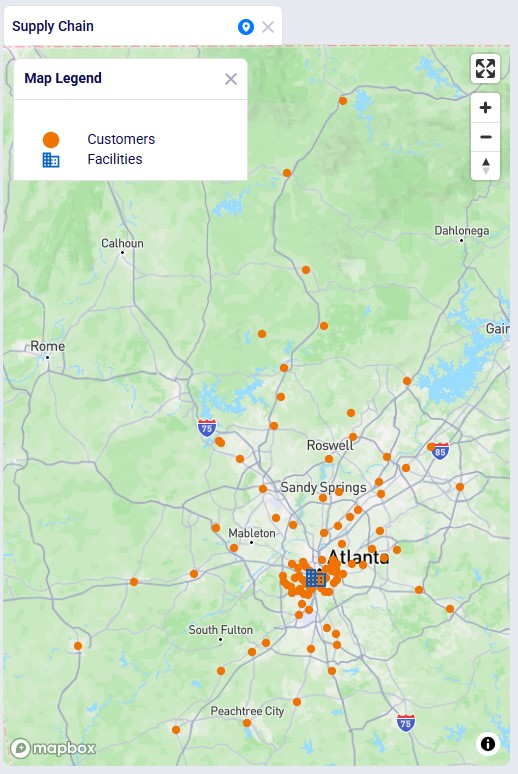
Let us also have a look at the customer and distribution center locations on the map before delving into the scenario details:
In this model, we will explore the following 4 scenarios:
To set up the predefined territories scenario, the Notes and Decomposition Name field on the Shipments table are used:
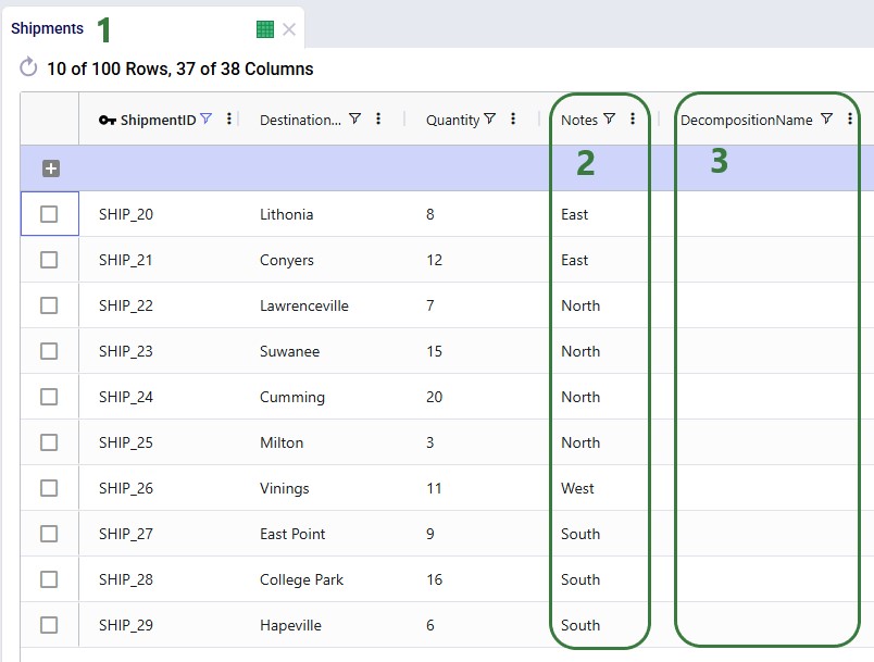
The configuration of the scenarios then looks as follows:
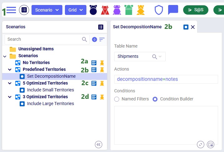
These scenarios are run with the Solver Focus Hopper model run option set to High Precision Mode as explained above.
Now, we will have a look at the outputs of these 4 scenarios and compare them. First, we will look at several output tables, including the 2 new ones. We will start with the Transportation Summary output table, which summarizes costs and other KPIs at the scenario level:
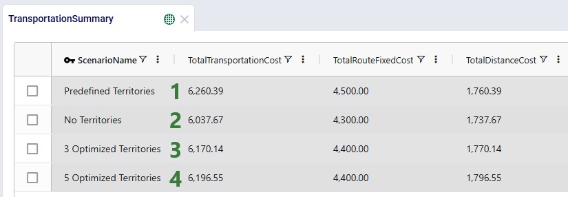
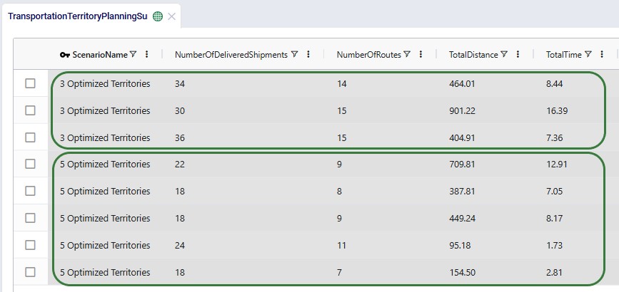
The next 2 screenshots are of the new Transportation Territory Planning Summary output table:
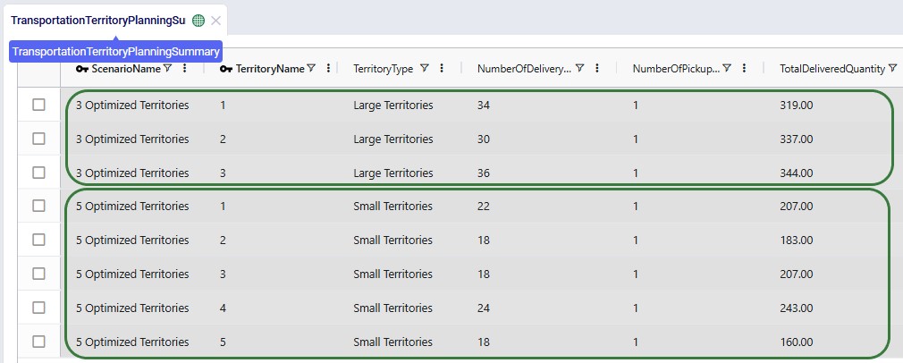
The top 3 records show the summarized outputs for each territory in the 3 Optimized Territories scenario, including the territory name and type, the number of delivery locations, the number of pickup locations, and the total delivered quantity. The bottom 5 records show the same outputs for the 5 territories of the 5 Optimized Territories scenario.
Scrolling right in this table shows additional outputs for each territory, including the number of delivered shipments, number of routes, total distance, and total time:
The other new output table, the Transportation Territory Assignment Summary table, contains the details of the assignments of customer locations to territories. The following screenshot shows the assignments of 6 customers in both the 3 Optimized Territories and 5 Optimized Territories scenarios:
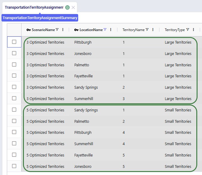
Please note that this table also includes the latitudes and longitudes of all customer locations (not shown in the screenshot), to allow easy visualization on a map.
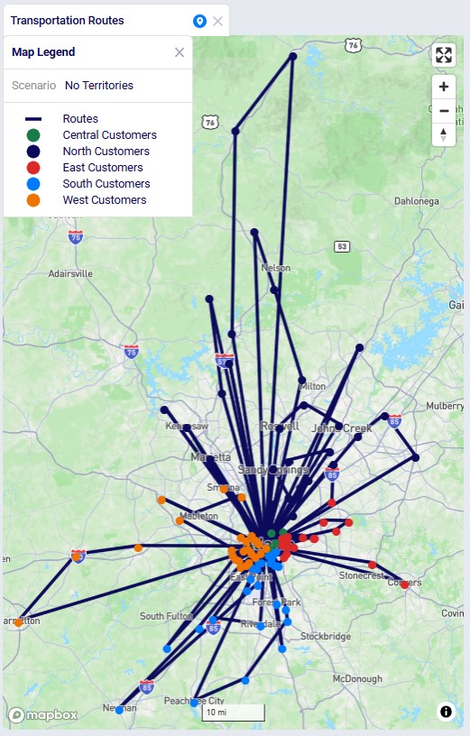
Next, we will have a look at the locations and routes on maps, these are also preconfigured in the template model that can be copied from the Resource Library, so you can have a look at these in Cosmic Frog yourself as well. The next screenshot shows the routes and locations of the Predefined Territories scenario on a map named Transportation Routes. The customers have been colored based on the predefined territory they belong to:
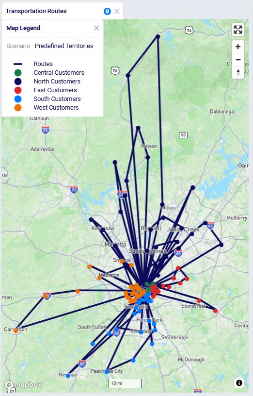
We can compare these routes to those of the No Territories scenario shown in the next screenshot. The customers are still colored based on the predefined territories, and if you zoom in a bit and pan through some routes, you will find several examples where customers from different predefined territories are now on a route together.
The following 2 screenshots compare the 3 and 5 Optimized Territories scenarios in a map called Territories Transportation Routes. The first shows the customers colored by territory. This is done by adding a layer to the map for each territory. The Transportation Stop Summary output table is used as the table to draw each of these "CZs Territory N" layers. Each layer's Condition Builder input uses "territoryname = 'N' and stoptype = 'Delivery'" as the filter; this is located on the layer's Condition Builder panel:
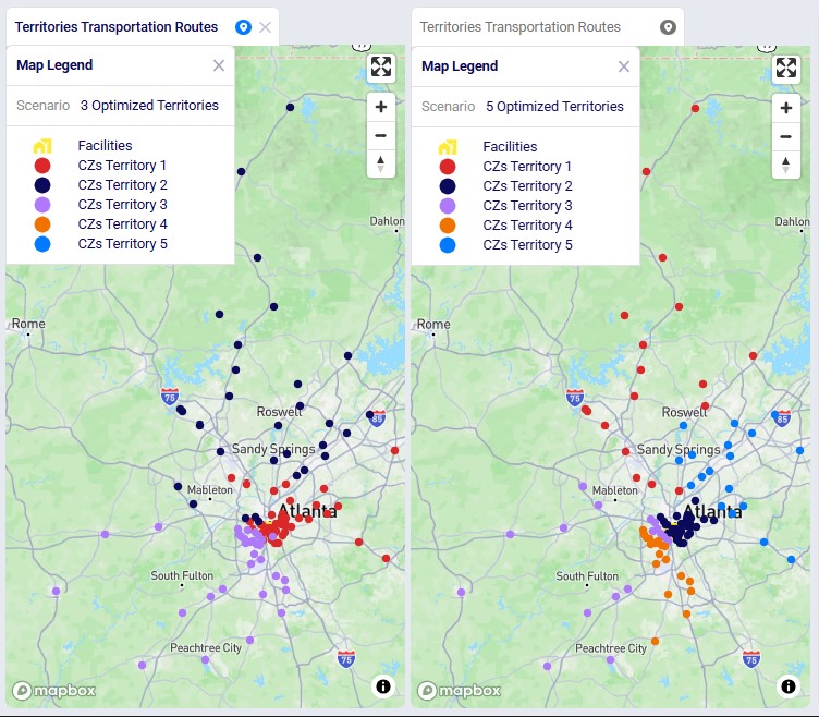
We see the customers clustered into their territories quite clearly in these visualizations. Some overlap between territories may happen, this can for example be due to non-uniform shipment sizes, pickup / delivery time windows, using actual road distances, etc.
This last screenshot shows the routes of the territories too, they are color coded based on the territory they belong too. This is done by again adding 1 map layer for each territory, this time drawing from the Transportation Routes Map layer table, and filtering in the Condition Builder for "territoryname = 'N'":
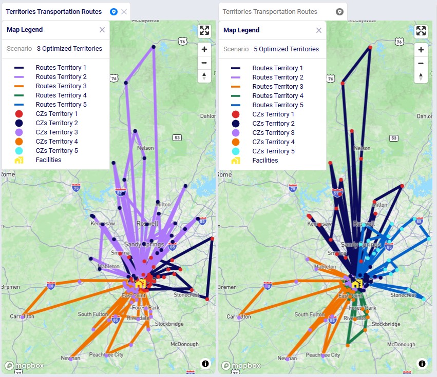
The Auto-Archiving feature helps keep your account clean and efficient while ensuring Optilogic maintains a streamlined, cost-effective storage footprint. By automatically archiving inactive databases, we reduce unnecessary server load, improve overall performance, and free up space so you can always create new Cosmic Frog models or DataStar projects when you need them.
From your perspective, Auto-Archiving means less manual cleanup and more confidence that your account is organized, fast, and ready for your next project.
Archiving moves a database from an active state into long-term storage. Once archived:
Important: Auto-archiving does not delete your data. You are always in control and can restore an archived database back into an active state.
With Auto-Archiving, you do not need to manually track and archive inactive databases. Our system will automatically archive any database that has been inactive for 90 days.
The screenshot below shows the notifications you will receive when 1) there are databases in your account that meet the criteria for an auto-archive event and 2) once databases have been archived:
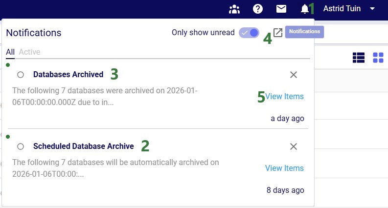
Now, we will take a look at the Notifications Page, which is opened using the pop-out icon in the in-app notification, described under bullet #4 above:
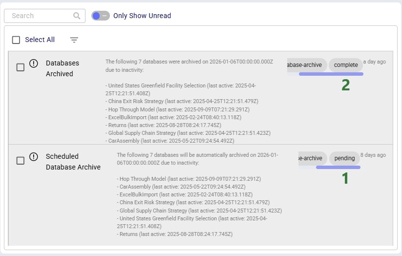
Clicking on the “View Items” link of a “Scheduled Database Archive” in-app notification (see bullet #5 of the first screenshot) will take you to a filtered view in the Cloud Storage application where you can see all the databases that will be auto-archived (note that this shows a different example with different databases to be archived as the previous screenshots):
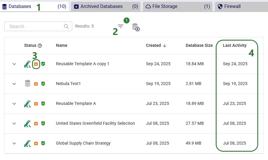
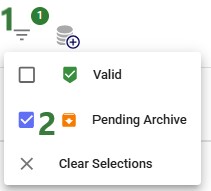
This next screenshot shows the filter that is applied on the Databases tab:
Clicking on the “View Items” link of a “Databases Archived” in-app notification (see bullet #5 of the first screenshot) will again take you to a filtered view in the Cloud Storage application where you can see the databases that have been auto-archived:
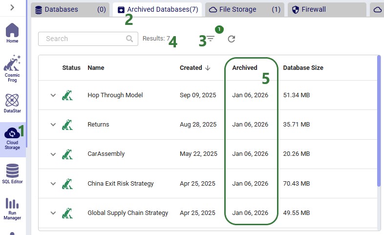
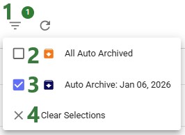
Finally, the following screenshot shows the filter that was applied on the Archived Databases tab:
Archiving is not just about organization — it also enhances performance across the platform. By reducing the number of idle databases consuming system resources, we lower the likelihood of “noisy neighbor” effects (when unused databases cause latency or compete with active ones).
With fewer inactive databases on high-availability servers, your active databases run faster and more reliably.
To keep a database active, simply interact with it. Any of the following actions will reset its inactivity timer:
Performing any of these actions ensures the database will not be archived.
Restoring an archived database is quick and straightforward:
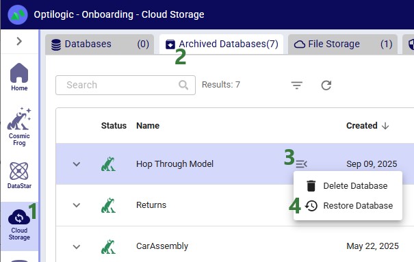
The system will start a background job to restore the database. You can track progress at any time on the Account Activity page.
What to expect:
Quota reminder: To unarchive a database, you will need enough space in your database quota. If you have already reached your limit, you may need to archive or delete another database before restoring.
Auto-Archiving helps you:
It is a simple, automated way to ensure your workspace stays efficient while protecting your data.
As always, please feel free to reach out to the Optilogic support team at support@optilogic.com for any questions or feedback.
Users of the Optilogic platform can easily access all files they have in their Optilogic account and perform common tasks like opening, copying, and sharing them by using the built-in Explorer application. This application sits across all other applications on the Optilogic platform.
This documentation will walk users through how to access the Explorer, explain its folder and file structure, how to quickly find files of interest, and how to perform common actions.
By default, the Explorer is closed when users are logged into the Optilogic platform, they can open it at the top of the applications list:

Once the Explorer is open, your screen will look similar to the following screenshot:
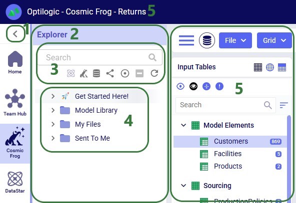
This next screenshot shows the Explorer when it is open while the user is working inside the workspace of one of the teams they are part of, and not in their My Account workspace:

When a new user logs into their Optilogic account and opens the Explorer, they will find there are quite a few folders and files present in their account already. The next screenshot shows the expanded top-level folders:
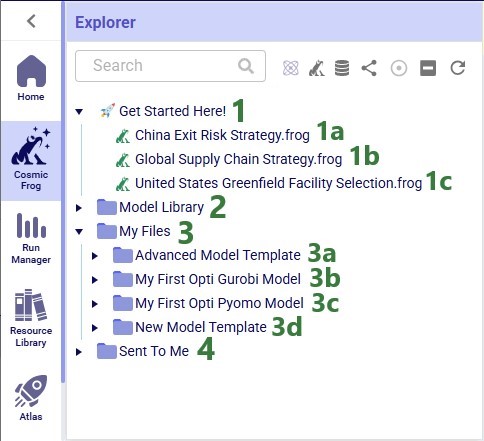
As you may have noticed already, different file types can be recognized by the different icons to the left of the file’s name. The following table summarizes some of the common file types users may have in their accounts, shows the icon used for these in the Explorer, and indicates which application the file will be opened in when (left-)clicking on the file:

*When clicking on files of these types, the Lightning Editor application will be opened and a message stating that the file is potentially unsupported will be displayed. Users can click on a “Load Anyway” button to attempt to load the file in the Lightning Editor. If the user chooses to do so, the file will be loaded, but the result will usually be unintelligible for these file types.
Some file types can be opened in other applications on the Optilogic platform too. These options are available from the right-click context menus, see the “Right-click Context Menus” section further below.
Icons to the right of names of Cosmic Frog models in the Explorer indicate if the model is a shared one and if so, what type of access the user / team has to it. Hovering over these icons will show text describing the type of share too.
Learn more about sharing models and the details of read-write vs read-only access in the “Model Sharing & Backups for Multi-user Collaboration in Cosmic Frog” help center article.
While working on the Optilogic platform, additional files and folders can be created in / added to a user’s account. In this section we will discuss which applications create what types of files and where in the folder structure they can be found in the Explorer.
The Resource Library on the Optilogic platform contains example Cosmic Frog models, DataStar template projects, Cosmic Frog for Excel Apps, Python scripts, reference data, utilities, and additional tools to help make Optilogic platform users successful. Users can browse the Resource Library and copy content from there to their own account to explore further (see the “How to use the Resource Library” help center article for more details):

Please note that Cosmic Frog models copied from the Resource Library are placed into a subfolder with the model’s name under the Resource Library folder; they can be recognized in the Explorer by their frog icon to the left of the model’s name and the .frog extension.
In addition, please note that previously, files copied from the Resource Library were placed in a different location in users’ accounts and not in the Resource Library folder and its subfolders. The old location was a subfolder with the resource’s name under the My Files folder. Users who have been using the Optilogic platform for a while will likely still see this file structure for files copied from the Resource Library before this change was made.
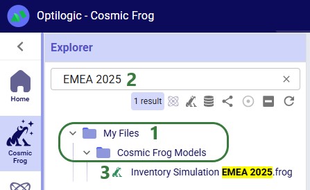
Users can create new Cosmic Frog models from Cosmic Frog’s start page (see this help center article); these will be placed in a subfolder named “Cosmic Frog Models”, which sits under the My Files folder:
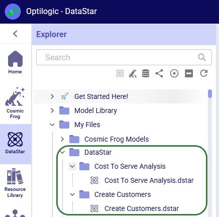
Users can create new DataStar projects from DataStar's start page (see this help center article); these will be placed in a subfolder named “DataStar”, which sits under the My Files folder. Within this DataStar folder, sub-folders with the names of the DataStar projects are created and the .dstar project files are located in these folders. In the following screenshot, we are showing 2 DataStar projects, 1 named "Cost to Serve Analysis" and 1 named "Create Customers":
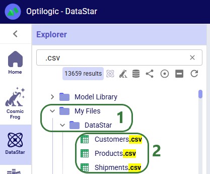
DataStar users may upload files to use with their data connections through the DataStar application (see this help center article). These uploaded files are also placed in the /My Files/DataStar folder:
When working with any of the Cosmic Frog for Excel Apps (see also this help center article), the working files for these will be placed in subfolders under the My Files folder. These are named “z Working Folder for … App”:
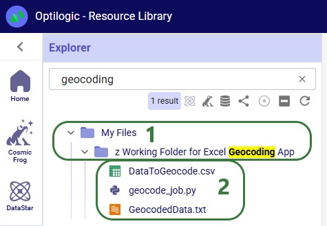
In addition to the above-mentioned subfolders (Resource Library, Cosmic Frog Models, DataStar, and “z Working Folder for … App” folders) which are often present under the My Files top-level folder in a user’s Optilogic account, there are several other folders worth covering here:
Now that we have covered the folder and file structure of the Explorer including the default and common files and folders users may find here, it is time to cover how users can quickly find what they need using the options towards the top of the Explorer application.
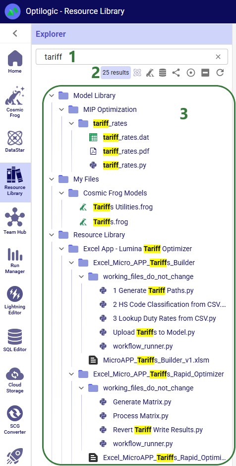
There is a free type text search box at the top of the Explorer application, which users can use to quickly find files and folders that contain the typed text in their names:
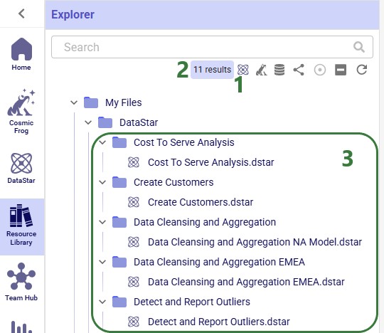
There is a quick search option to find all DataStar projects in the user’s account:
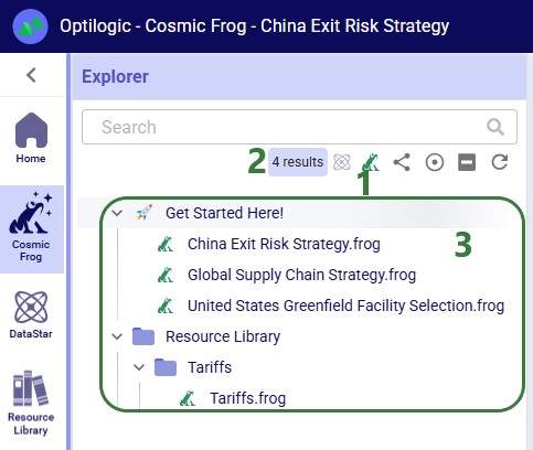
Similarly, there is a quick search option to find all Cosmic Frog models in the user’s account:
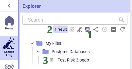
There is also a quick filter function to find all PostgreSQL databases in a user's account:
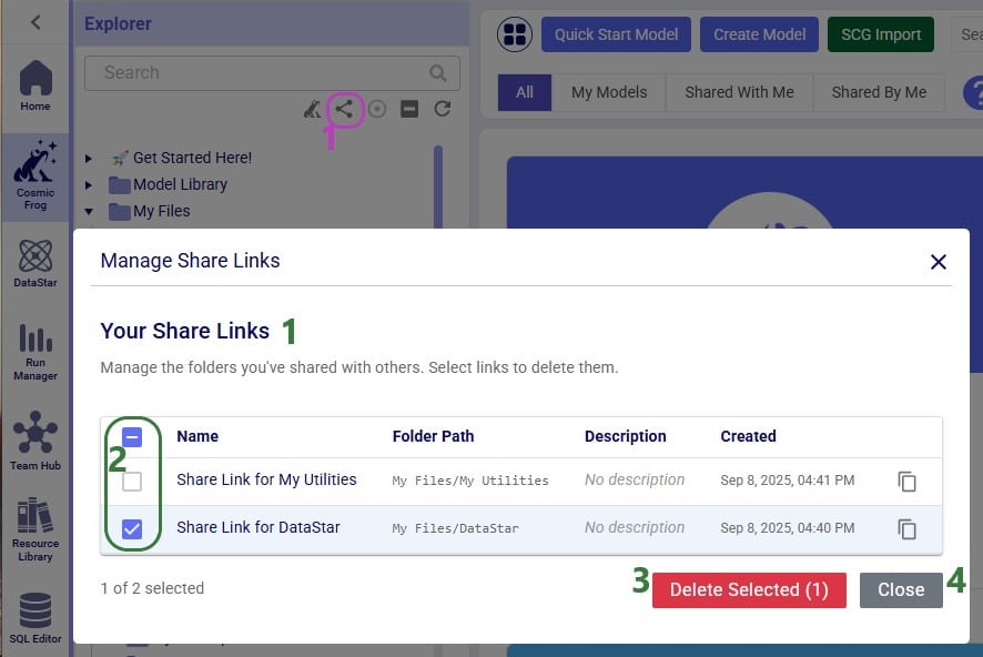
Users can create share links for folders in their Optilogic account to send a copy of the folder and all its contents to other users. See this “Folder Sharing” section in the “Model Sharing & Backups for Multi-User Collaboration in Cosmic Frog” help center article on how to create and use share links. If a user has created any share links for folders in their account, these can be managed by clicking on the View Share Links icon:
When browsing through the files and folders in your Optilogic account, you may collapse and expand quite a few different folders and their subfolders. Users can at times lose track of where the file they had selected is located. To help with this, users have the “Expand to Selected File” option available to them:
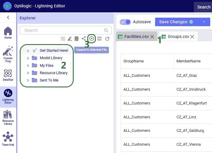
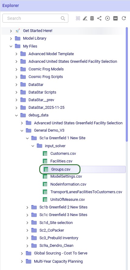
In addition to using the Expand to Selected File option, please note that switching to another file in the Lightning Editor by for example clicking on the Facilities.csv file, will further expand the Explorer to show that file in the list too. If needed, the Explorer will also automatically scroll up or down to show the active file in the center of the list.
If you have many folders and subfolders expanded, it can be tedious to collapse them all one by one again. Therefore, users also have a “Collapse All” option at their disposal when working with the Explorer. The following screenshot shows the state of the Explorer before clicking on the Collapse All icon, which is the 6th of the 7 icons to the right of the Search box in the following screenshot:
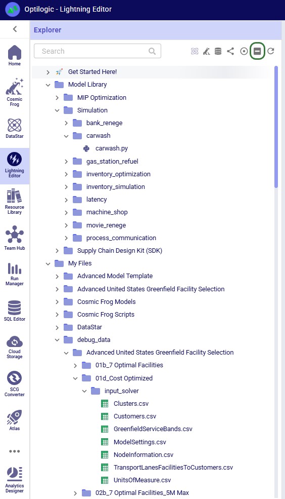
The user then clicks on the Collapse All icon and the following screenshot shows the state of the Explorer after doing so:

Note that the Collapse All icon has now become inactive and will remain so until any folders are expanded again.
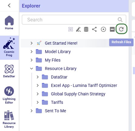
Sometimes when deleting, copying, or adding files or folders to a user’s account, these changes may not be immediately reflected in the Explorer files & folders list as they may take a bit of time. The last of the icons to the right of / underneath the Search box provides users with a “Refresh Files” option. Clicking on this icon will update the files and folders list such that all the latest are showing in the Explorer:
In this final section of the Explorer documentation, we will cover the options users have from the context menus that come up when right-clicking on files and folders in the Explorer. Screenshots and text will explain the options in the context menus for folders, Cosmic Frog models, text-based files, and all other files.
When right-clicking on a folder in the Explorer, users will see the following context menu come up (here the user right-clicked on the Model Library folder):
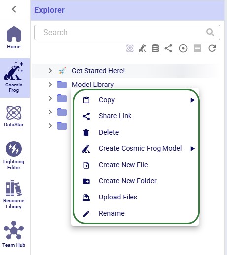
The options from this context menu are, from top to bottom:
Note that right-clicking on the Get Started Here folder gives fewer options: just the Copy (with the same 3 options as above), Share Link, and Delete Folder options are available for this folder.
Now, we will cover the options available from the context menu when right-clicking on different types of files, starting with Cosmic Frog models:

The options, from top to bottom, are:
Please note that the Cosmic Frog models listed in the Explorer are not actual databases, but pointer files. These are essentially empty placeholder files to let users visualize and interact with models inside the Explorer. Due to this, actions like downloading are not possible; working directly with the Cosmic Frog model databases can be done through Cosmic Frog or the SQL Editor.
Next, we will look at the right-click context menu for DataStar projects. The options here are very similar to those of Cosmic Frog models:
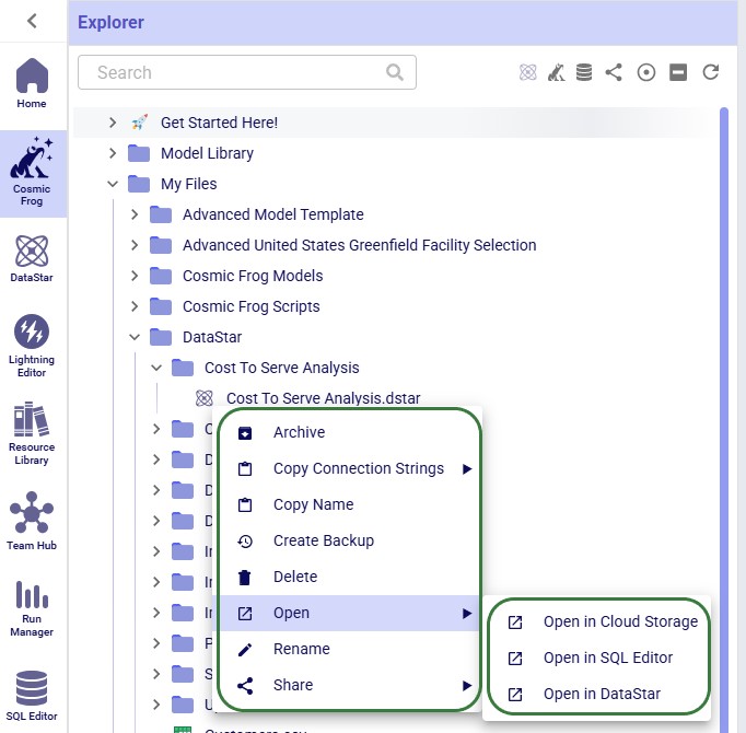
The options, from top to bottom, are:
When right-clicking on a Python script file, the following context menu will open:
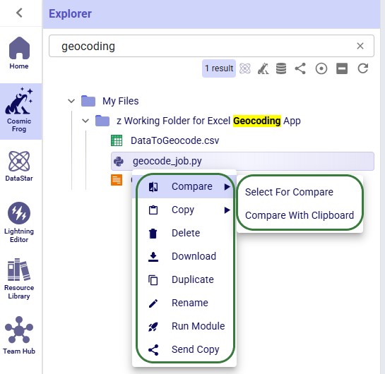
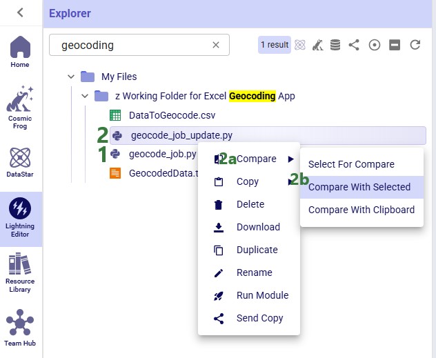
The options, from top to bottom, are:
The next 2 screenshots show what it looks like when comparing 2 text-based files with each other:
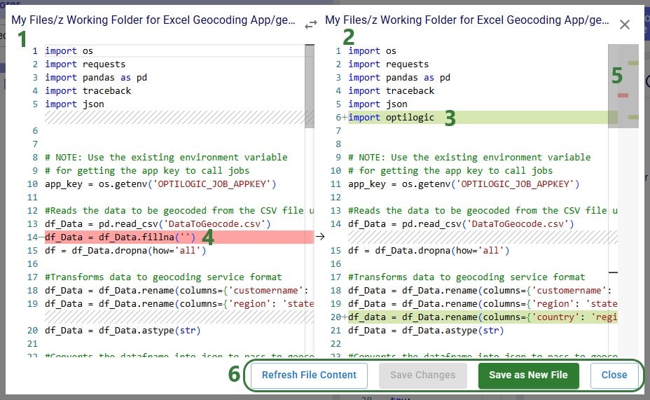
Other text-based files, such as those with extensions of .csv, .txt, .md and .html have the same options in their context menus as those for Python script files, with the exception that they do not have a Run Module option. The next screenshot shows the context menu that comes up when right-clicking on a .txt file:

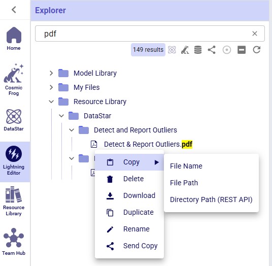
Other files, such as those with extensions of .pdf, .xls, .xlsx, .xlsm, .png, .jpg, .twb and .yxmd, have the same options from their context menus as Python scripts, minus the Compare and Run Module options. The following screenshot shows the context menu of a .pdf file:
As always, please feel free to let us know of any questions or feedback by contacting Optilogic support on support@optilogic.com.
This documentation covers which geo providers one can use with Cosmic Frog, and how they can be used for geocoding and distance and time calculations.
Currently, there are 5 geo providers that can be used for geocoding locations in Cosmic Frog: MapBox, Bing, Google, PTV, and PC*Miler. MapBox is the default provider and comes free of cost with Cosmic Frog. To use any of the other 4 providers, you will need to obtain a license key from the company and add this to Cosmic Frog through your Account. The steps to do so are described in this help article “Using Alternate Geocoding Providers”.
Different geocoding providers may specialize in different geographies; refer to your provider for guidelines.
Geocoding a location (e.g. a customer, facility or supplier) means finding the latitude and longitude for it. Once a location is geocoded it can be shown on a map in the correct location which helps with visualizing the network itself and building a visual story using model inputs and outputs that are shown on maps.

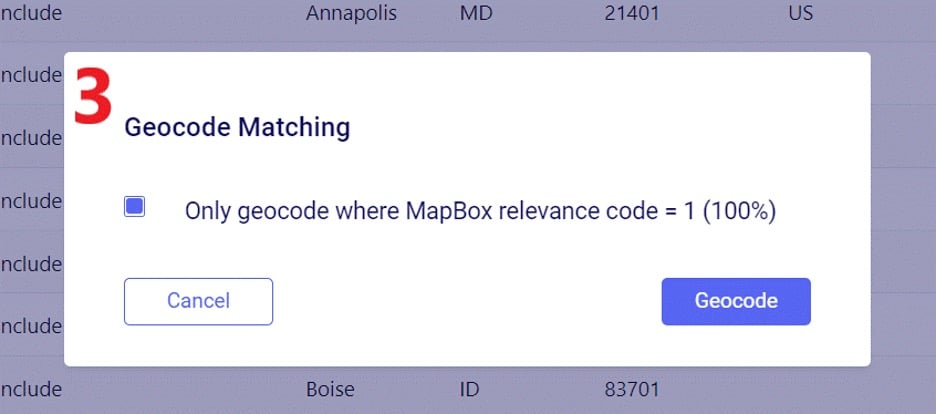
To geocode a location:
For costs and capacities to be calculated correctly, it may be needed to add transport distances and transport times to Cosmic Frog models. There are defaults that will be used if nothing is entered into the model, or users can populate these fields, either themselves or by using a Distance Lookup Utility. Here the tables where distances and times can be entered, what happens if nothing has been entered, and how users can utilize the Distance Lookup Utility will be explained.
There are multiple Cosmic Frog input tables that have input fields related to Transport Distance, and Transport Time, including Speed which can also be used to calculate transport time from a Transport Distance (time = distance / speed). These all have their own accompanying UOM (unit of measure) field. Here is an overview of the tables which contain Distance, Time and/or Speed fields:

For Optimization (Neo), this is the order of precedence that is applied when multiple tables and fields are used:
For Transportation (Hopper) models, this is the order of precedence when multiple tables and fields are being used:
To populate these input tables and their pertinent fields, user has following options:
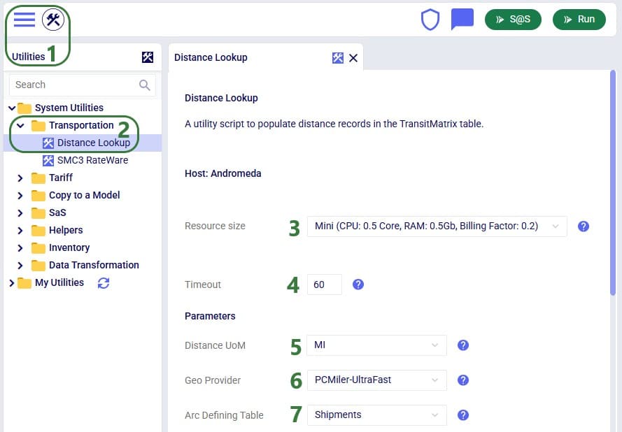
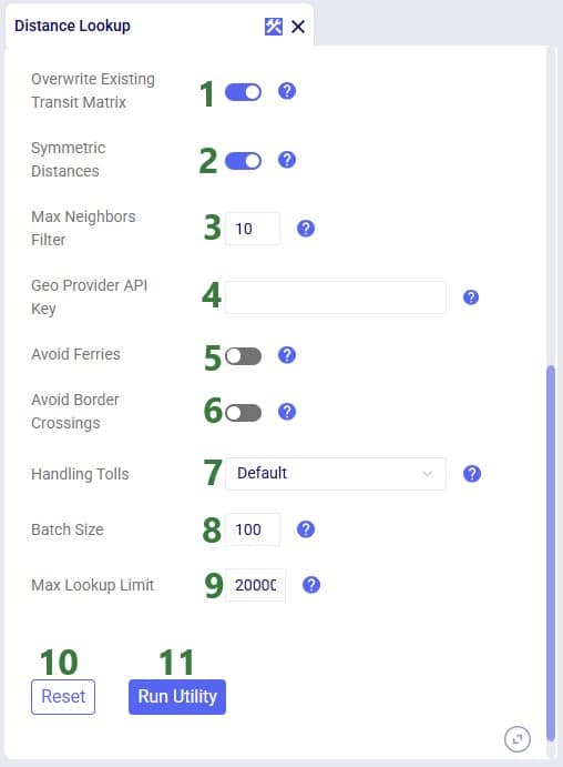
Cosmic Frog users can find multiple handy utilities in the Utilities section of Cosmic Frog - here we will cover the Distance Lookup utility. This utility looks up transportation distances and times for origin-destination pairs and populates the Transit Matrix table. As Geo Providers, Bing, PC Miler and Azure can be used if the user has a license key for these. In addition, there is a free PC Miler-UltraFast option which can look up accurate road distances within the EU and North America without needing a license key. This is also a very fast way to lookup distances. A new free provider OLRouting has been added. This provider leverages valhalla, an open source routing engine for OpenStreetMap. It has global coverage and performs the lookups very fast as well. Lastly, the Great Circle Geo Provider option calculates the straight-line distance for origin-destination pairs based on latitudes & longitudes. We will look at the configuration options of the utility using the next 2 screenshots:
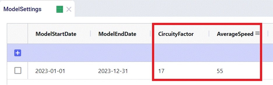
Note that when using the Great Circle geo provider for Distance calculations, only the Transport Distance field in the Transit Matrix table will be populated. The Transport Time will be calculated at run time using the Average Speed on the Model Settings table.
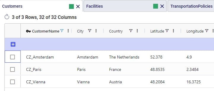
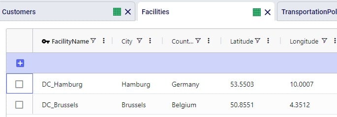
To finish up, we will walk through an example of using the Distance Lookup utility on a simple model with 3 customers (CZs) and 2 distribution centers (DCs), which are shown in the following 2 screenshots of the Customers and Facilities tables:
We can use Groups and/or Named Table Filters in the Transportation Policies table if we want to make 1 policy that represents all possible lanes from the DCs to the customers:

Next, we run the Distance Lookup utility with following settings:
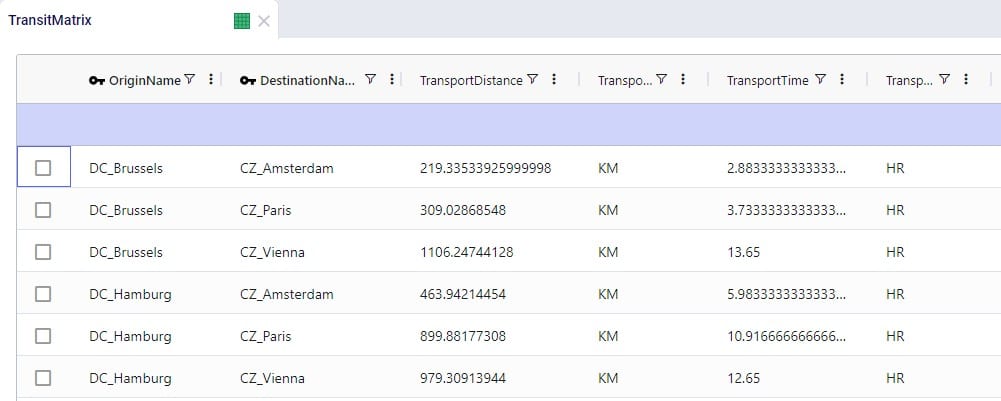
This results in the following 6 records being added to the Transit Matrix table - 1 for each possible DC-CZ origin-destination pair:
Cosmic Frog’s new breakpoints feature enables users to create maps which relay even more supply chain data in just one glance. Lines and points can now be styled based on field values from the underlying input or output table the lines/points are drawn from.
In this Help Center article, we will cover where to find the breakpoints feature for both point and line layers and how to configure them. A basic knowledge of how to configure maps and their layers in Cosmic Frog is assumed; users unfamiliar with maps in Cosmic Frog are encouraged to first read the “Getting Started with Maps” Help Center article.
First, we will walk through how to apply breakpoints to map layers of type = line, which are often used to show flows between locations. With breakpoints we can style the lines between origins and destinations for example based on how much is flowing in terms of quantity, volume or weight. It is also possible to style the lines on other numeric fields, like costs, distances or time.
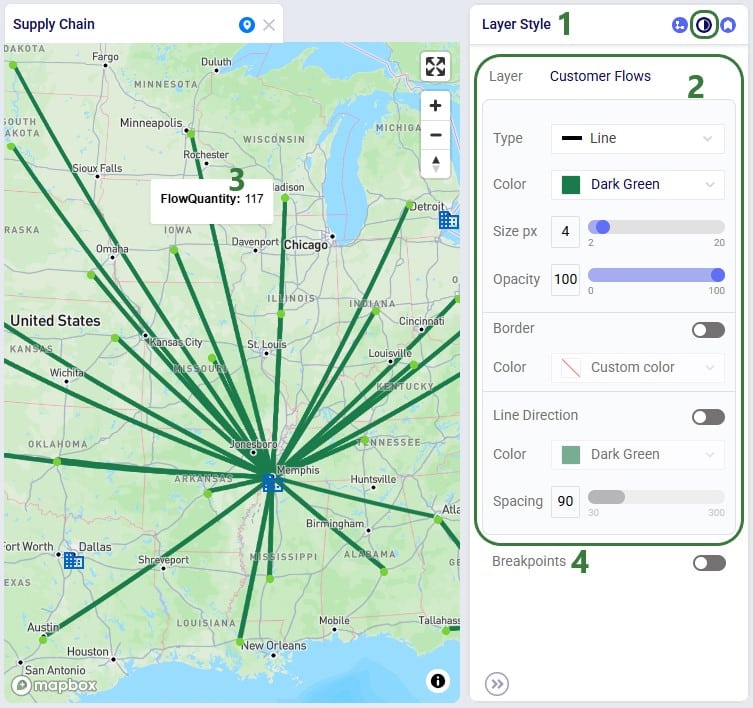
Consider the following map showing flows (dark green lines) to customers (light green circles):
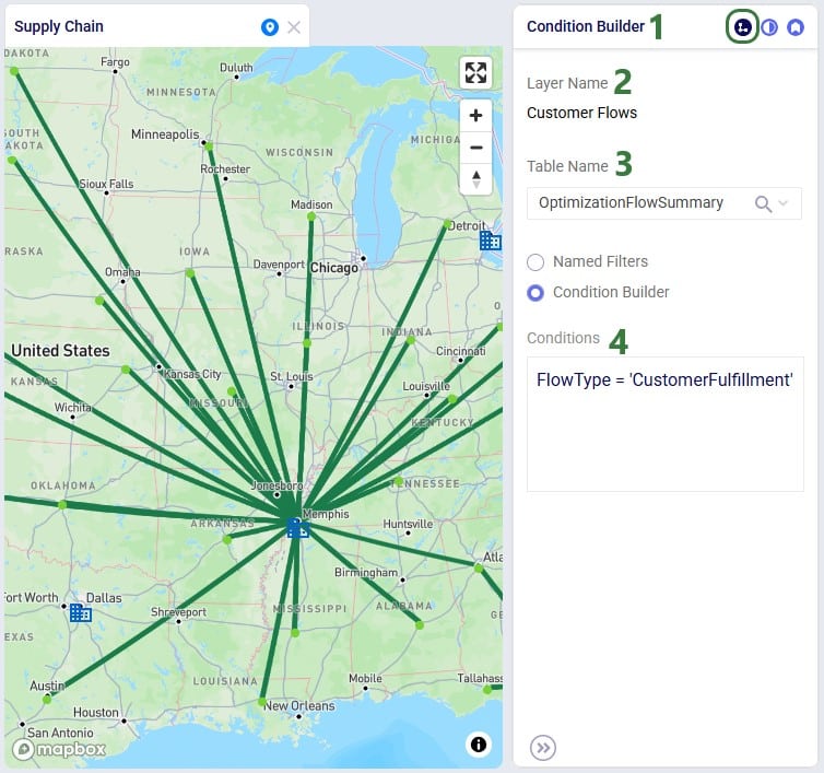
Next, we will go to the Layer Style pane on which breakpoints can be turned on and configured:
Once the Breakpoints toggle has been turned on (slide right, the color turns blue), the breakpoint configuration options become visible:
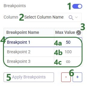
One additional note is that one can use tab to navigate through the cells in the Breakpoints table.
The next screenshot shows breakpoints based on the Flow Quantity field (in the Optimization Flow Summary) for which the Max Values have been auto generated:
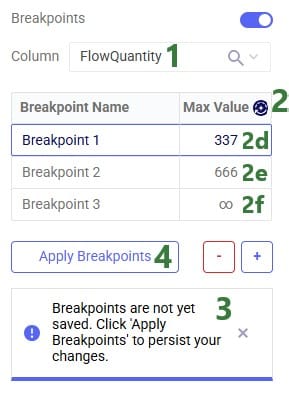
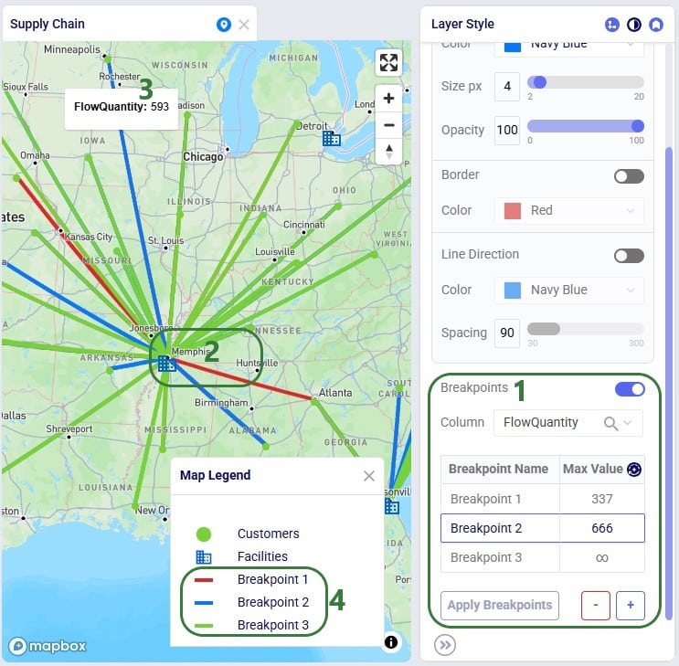
Users can customize the style of each individual breakpoint:

Please note:
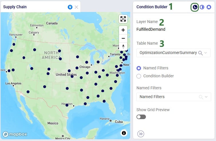
Configuring and applying breakpoints on point layers is very similar to those on line layers. We will walk through the steps in the next 4 screenshots in slightly less detail. In this example we will base the size of the customer locations on the map on the total demand they have been served:
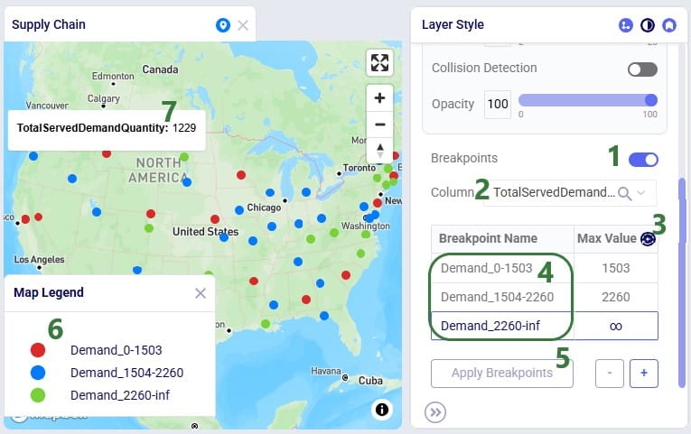
Next, we again look at the Layer Style pane of the layer:

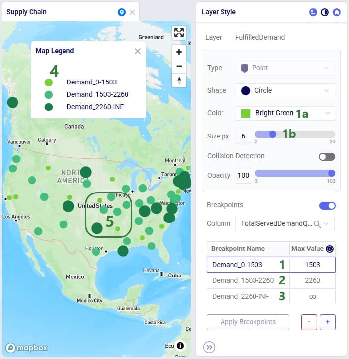
Lastly, user would like to gradually increase the color of the customer circles from light to dark green and the size from small to bigger based on the breakpoint the customer belongs to:
As always, please feel free to reach out to Optilogic support at support@optilogic.com should you have any questions.
For various reasons, many supply chains need to deal with returns. This can for example be due to packaging materials coming back to be reused at plants or DCs, retail customers returning finished goods that they are not happy with, defective products, etc. Previously, these returns could mostly be modelled within Cosmic Frog NEO (Network Optimization) models by using some tricks and workarounds. But with the latest Cosmic Frog release, returns are now supported natively, so that the reuse, repurposing, or recycling of these retuned products to help companies reduce costs, minimize waste, and improve overall supply chain efficiency can be taken into account easily.
This documentation will first provide an overview of how returns work in a Cosmic Frog model and then walk through an example model of a retailer which includes modelling the returns of finished goods. The appendix details all the new returns-related fields in several new tables and some of the existing tables.
When modelling returns in Cosmic Frog:
Users need to use 2 new input tables to set up returns:
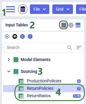
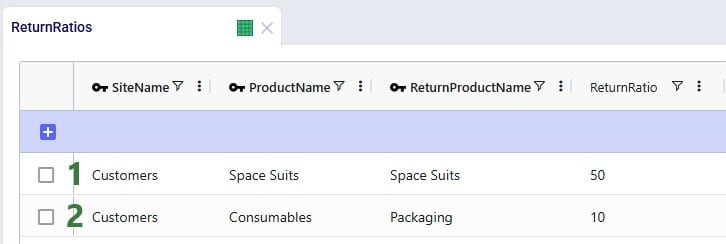
The Return Ratios table contains the information on how much return-product is returned for a certain amount of product delivered to a certain destination:
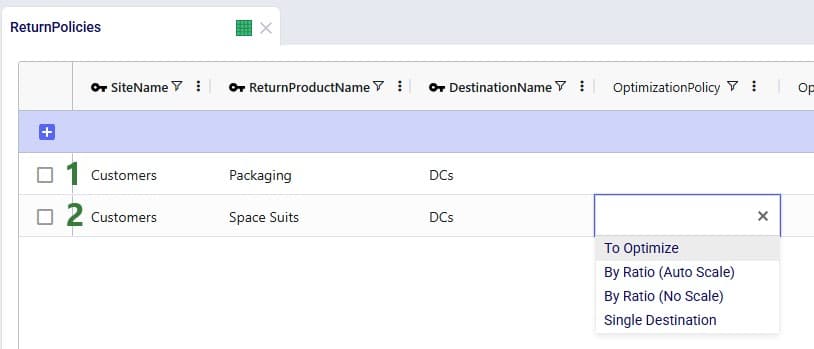
The Return Policies table is used to indicate where returned products need to go to and the rules around multiple possible destinations. Optionally, costs can be associated with the returns here and a maximum distance allowed for returns can be entered on this table too.
Note that both these tables have Status and Notes fields (not shown in the screenshots), like most Cosmic Frog input tables have. These are often used for scenario creation where the Status is set to Exclude in the table itself and changed to Include in select scenarios based on text in the Notes field.
All columns on these 2 returns-related input table are explained in more detail in the appendix.
In addition to populating the Return Policies and Return Ratios tables, users need to be aware that additional model structure needed for the returned products may need to be put in place:
The Optimization Return Summary output table is a new output table that will be generated for Neo runs if returns are included in the modelling:
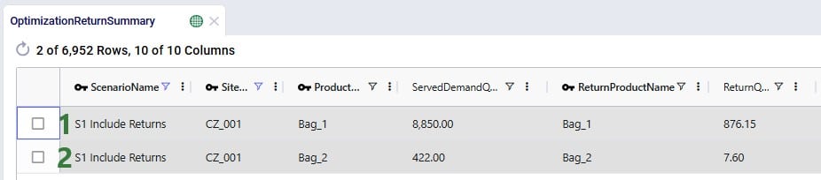
This table and all its fields are explained in detail in the appendix.
The Optimization Flow Summary output table will contain additional records for models that include returns; they can be identified by filtering the Flow Type field for “Return”:

These 2 records show the return flows and associated transportation costs for the Bag_1 and Bag_2 products from CZ_001, going to DC_Cincinnati, that we saw in the Optimization Return Summary table screenshot above.
In addition to the new Optimization Return Summary output table, and new records of Flow Type = Return in the Optimization Flow Summary output table, following existing output tables now contain additional fields related to returns:
The example Returns model can be copied from the Resource Library to a user’s Optilogic account (see this help center article on how to use the Resource Library). It models the US supply chain of a fashion bag retailer. The model’s locations and flows both to customers and between DCs are shown in this screenshot (returns are not yet included here):
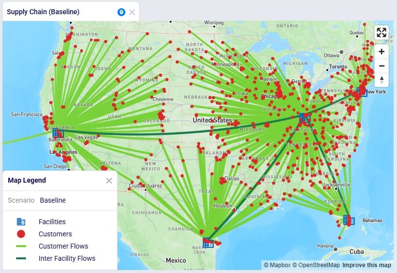
Historically, the retailer had 1 main DC in Cincinnati, Ohio, where all products were received and all 869 customers were fulfilled from. Over time, 4 secondary DCs were added based on Greenfield analysis, 2 bigger ones in Clovis, California, and Jersey City, New Jersey, and 2 smaller ones in West Palm Beach, Florida, and Las Lomas, Texas. These secondary DCs receive product from the Cincinnati DC and serve their own set of customers. The main DC in Cincinnati and the 2 bigger secondary DCs (Clovis, CA, and Jersey City, NJ) can handle returns currently: returns are received there and re-used to fulfill demand. However, until now, these returns had not been taken into account in the modelling. In this model we will explore following scenarios:
Other model features:
Please note that in this model the order of columns in the tables has sometimes been changed to put those containing data together on the left-hand side of the table. All columns are still present in the table but may be in a different position than you are used to. Columns can be reset to their default position by choosing “Reset Columns” from the menu that comes up when clicking on the icon with 3 vertical dots to the right of a column name.
After running the baseline scenario (which does not include returns), we take a look at the Financials: Scenario Cost Comparison chart in the Optimization Scenario Comparison dashboard (in Cosmic Frog’s Analytics module):
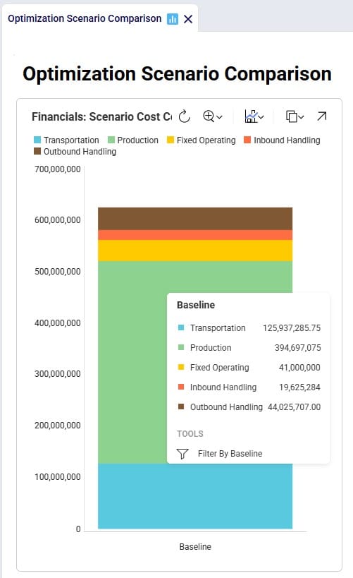
We see that the biggest cost currently is the production cost at 394.7M (= procurement of all product into Cincinnati), followed by transportation costs at 125.9M. The total supply chain cost of this scenario is 625.3M.
In this scenario we want to include how returns currently work: Cincinnati, Clovis, and Jersey City customers return their products to their local DCs whereas West Palm Beach and Las Lomas customers return their products to the main DC in Cincinnati. To set this up, we need to add records to the Return Policies, Return Ratios, and Transportation Policies input tables. To not change the Baseline scenario, all new records will be added with Status = Exclude, and the Notes field populated so it can be used to filter on in scenario items that change the Status to Include for subsets of records. Starting with the Return Policies table:
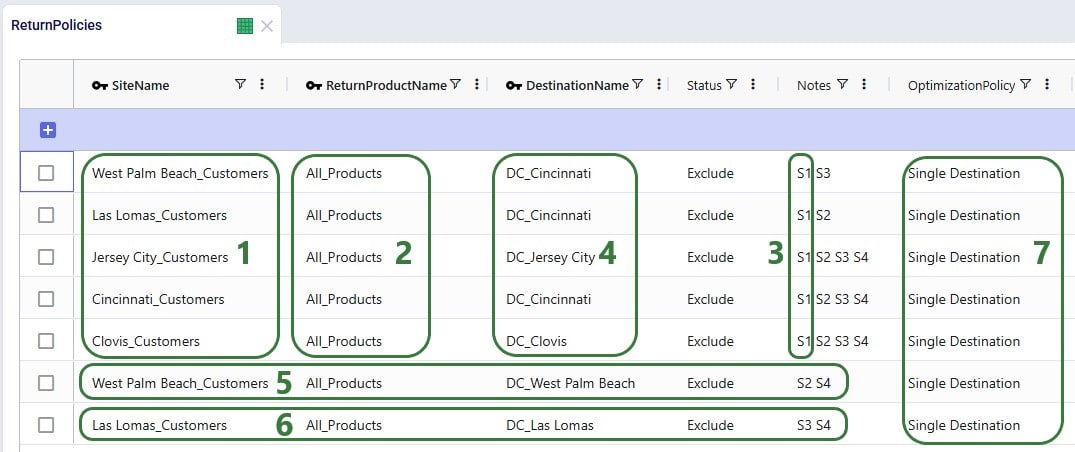
Next, we need to add records to the Transportation Policies table so that there is at least 1 lane available for each site-product-destination combination set up in the return policies table. For this example, we add records to the Transportation Policies table that match the ones added to the Return Policies table exactly, while additionally setting Mode Name = Returns, Unit Cost = 0.04 and Unit Cost UOM = EA-MI (the latter is not shown in the screenshot below), which means the transportation cost on return lanes is 0.04 per unit per mile:
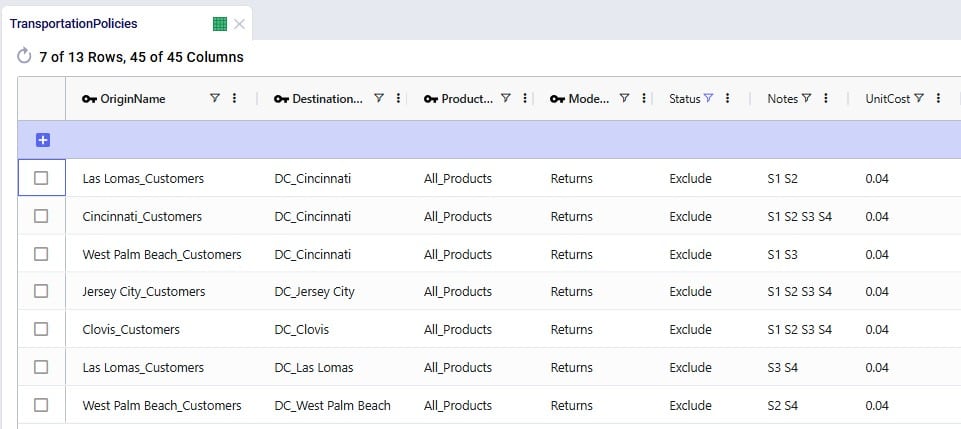
Finally, we also need to indicate how much product is returned in the Return Ratios table. Since we want to model different ratios by individual customer and individual product, this table does not use any groups. Groups can however be used in this table too for the Site Name, Product Name, Period Name, and Return Product Name fields.
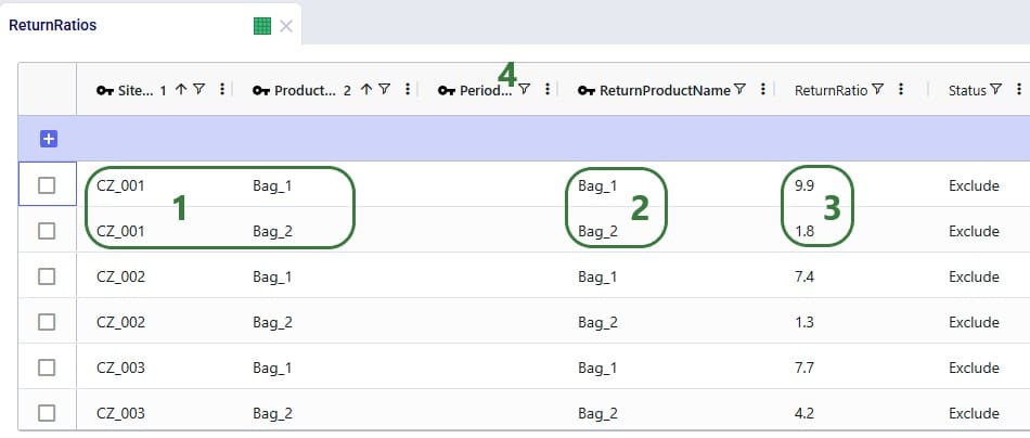
Please note that adding records to these 3 tables and including them in the scenarios is sufficient to capture returns in this example model. For other models it is possible that additional tables may need to be used, see the Other Input Tables section above.
Now that we have populated the input tables to capture returns, we can set up scenario S1 which will change the Status of the appropriate records in these tables from Exclude to Include:
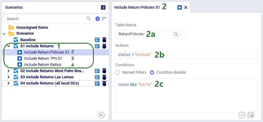
After running this scenario S1, we are first having a look at the map, where we will be showing the DCs, Customers and the Return Flows for scenario S1. This has been set up in the map named Supply Chain (S1) in the model from the Resource Library. To set this map up, we first copied the Supply Chain (Baseline) map and renamed it to Supply Chain (S1). Then clicked on the map’s name (Supply Chain (S1)) to open it and in the Map Filters form that is showing on the right-hand side of the screen changed the scenario to “S1 Include Returns” in the Scenario drop-down. To configure the Return Flows, we added a new Map Layer, and configured its Condition Builder form as follows (learn more about Maps and how to configure them in this Help Center article):
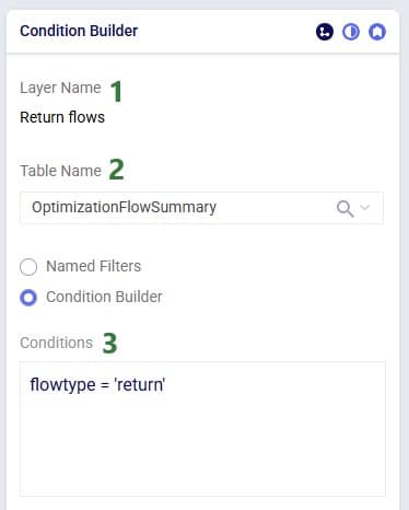
The resulting map is shown in this next screenshot:
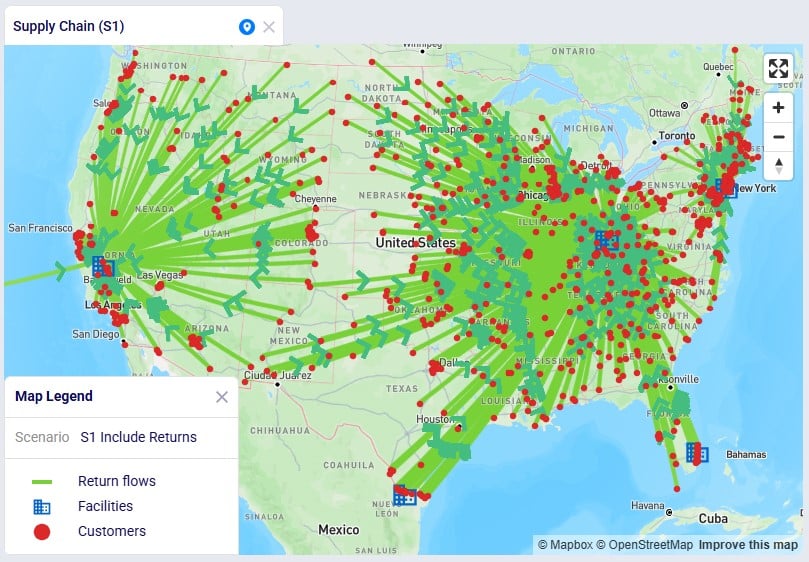
We see that, as expected, the bulk of the returns are going back the main DC in Cincinnati: from its local customers, but also from the customers served by the 2 smaller DCs in Las Lomas and West Palm Beach DCs. The customers served by the Clovis and Jersey City DCs return their products to their local DCs.
To assess the financial impact of including returns in the model, we again look at the Financials: Scenario Cost Comparison chart in the Optimization Scenario Comparison dashboard, comparing the S1 scenario to the Baseline scenario:

We see that including returns in S1 leads to:
Seeing that the main driver for the overall supply chain costs being higher when including returns are the high transportation costs for returning products, especially those travelling long distances from the Las Lomas and West Palm Beach customers to the Cincinnati DC sparks the idea to explore if it would be more beneficial for the Las Lomas and/or West Palm Beach customers to return their products to their local DC, rather than the Cincinnati DC. This will be modelled in the next three scenarios.
Building upon scenario S1, we will run 2 scenarios (S2 and S3) where it will be examined if it is beneficial cost-wise for West Palm Beach customers to return their products to their local West Palm Beach DC (S2) and for Las Lomas customers to return their products to their local Las Lomas DC (S3) rather than to the Cincinnati DC. In order to be able to handle returns, the fixed operating costs at these DCs are increased by 0.5M to 3.5M:

Scenarios S2 and S3 are run, and first we look at the map to check the return flows for the West Palm Beach and Las Lomas customers, respectively (copied the map for S1, renamed it, and then changed the scenario by clicking on the map’s name and selecting the S2/S3 scenario from the Scenario drop-down in the Map Filters pane on the right-hand side):
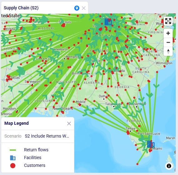
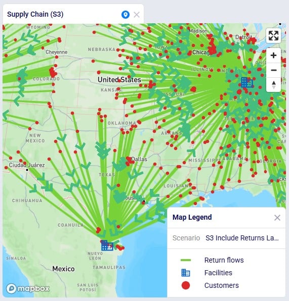
As expected, due to how we set up these scenarios, now all returns from these customers go to their local DC, rather than to DC-Cincinnati which was the case in scenario S1.
Let us next look at the overall costs for these 2 scenarios and compare them back to the S1 and Baseline scenarios:
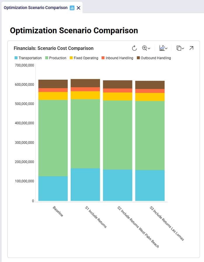
Besides some smaller reductions in the inbound and outbound costs in S2 and S3 as compared to S1, the transportation costs are reduced by sizeable amounts: 6.9M (S2 compared to S1) and 9.4M (S3 compared to S1), while the production (= procurement) costs are the same across these 3 scenarios. The reduction in transportation costs outweighs the 0.5M increase in fixed operating costs to be able to handle returns at the West Palm Beach and Las Lomas DCs. Also note that both scenario S2 and S3 have a lower total cost than the Baseline scenario.
Since it is beneficial to have the West Palm Beach and Las Lomas DCs handle returns, scenario S4 where this capability is included for both DCs is set up and run:
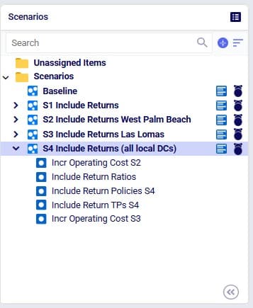
The S4 scenario increases the fixed operating costs at both these DCs from 3M to 3.5M (scenario items “Incr Operating Cost S2” and “Incr Operating Cost S3”), sets the Status of all records on the Return Ratios table to Include (the Include Return Ratios scenario item), and sets the Status to Include for records on the Return Policies and Transportation Policies tables where the Notes field contains the text “S4” (the “Include Return Policies S4” and “Include Return TPs S4” items), which are records where customers all ship their returns back to their local DC. We first check on the map if this is working as expected after running the S4 scenario:
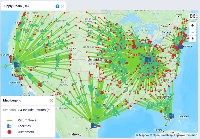
We notice that indeed there are no more returns going back to the Cincinnati DC from Las Lomas or West Palm Beach customers.
Finally, we expect the costs of this scenario to be the lowest overall since we should see the combined reductions of scenarios S2 and S3:
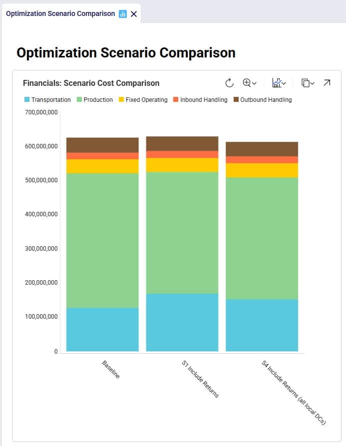
Between S1 and S4:
In addition to looking at maps or graphs, users can also use the output tables to understand the overall costs and flows, including those of the returns included in the network.
Often, users will start by looking at the overall cost picture using the Optimization Network Summary output table, which summarizes total costs and quantities at the scenario level:
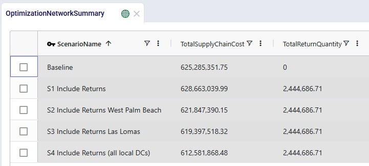
For each scenario, we are showing the Total Supply Chain Cost and Total Return Quantity fields here. As mentioned, the Baseline did not include any returns, whereas scenarios S1-4 did, which is reflected in the Total Return Quantity values. There are many more fields available on this output table, but in the next screenshot we are just showing the individual cost buckets that are used in this model (all other cost fields are 0):
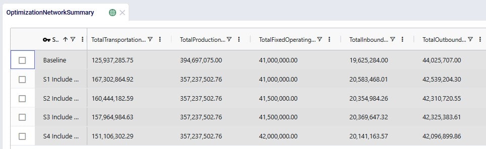
How these costs increase/decrease between scenarios has been discussed above when looking at the “Financials: Scenario Cost Comparison” chart in the “Optimization Scenario Comparison” dashboard. In summary:
Please note that on this table, there is also a Total Return Cost field. It is 0 in this example model. It would be > 0 if the Unit Cost field on the Return Policies table had been populated, which is a field where any specific cost related to the return can be captured. In our example Returns model, the return costs are entirely captured by the transportation costs and fixed operating costs specified.
The Optimization Return Summary output table is a new output table that has been added to summarize returns at the scenario-returning site-product-return product-period level:
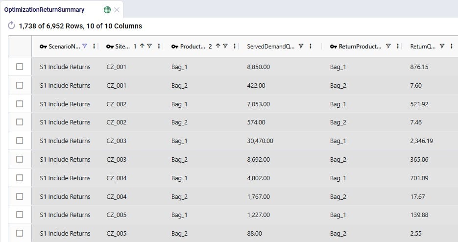
Looking at the first record here, we understand that in the S1 scenario, CZ_001 was served 8,850 units of Bag_1, while 876.15 units of Bag_1 were returned.
Lastly, we can also see individual return flows in the Optimization Flow Summary table by filtering the Flow Type field for “Return”:
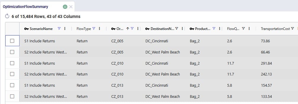
Note that the product name for these flows is of the product that is being returned.
The example Returns model described above assumes that 100% of the returned Bag_1 and Bag_2 products can be reused. Here we will discuss through screenshots how the model can be adjusted to take into account that only 70% of Bag_1 returns and 50% of Bag_2 returns can be reused. To achieve this, we will need to add an additional “return” product for each finished good, set up bills of materials, and add records to the policies tables for the required additional model structure.
The tables that will be updated and for which we will see a screenshot each below are: Products, Groups, Return Policies, Return Ratios, Transportation Policies, Warehousing Policies, Bills of Materials, and Production Policies.
Two products are added here, 1 for each finished good: Bag_1_Return and Bag_2_Return. This way we can distinguish the return product from the sellable finished goods, apply different policies/costs to them, and convert a percentage back into the sellable items. The naming convention of adding “_Return” to the finished good name makes for easy filtering and provides clarity around what the product’s role is in the model. Of course, users can use different naming conventions.
The same unit value as for the finished goods is used for the return products, so that inventory carrying cost calculations are consistent. A unit price (again, same as the finished goods) has been entered too, but this will not actually be used by the model as these “_Return” products are not used to serve customer demand.

To facilitate setting up policies where the return products behave the same (e.g. same lanes, same costs, etc.), we add an “All_Return_Products” group to the Groups table, which consists of the 2 return products:
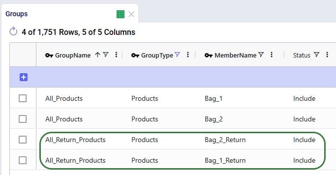
In the Return Policies table, the Return Product Name column needs to be updated to reflect that the products that are being returned are the “_Return” products. Previously, the Return Product Name was set to the All_Products group for each record, and it is now updated to the All_Return_Products group. Updating a field in all records or a subset of filtered records to the same value can be done using the Bulk Update Column functionality, which can be accessed by clicking on the icon with 3 vertical dots to the right of the column name and then choosing “Bulk Update this Column” in the list of options that comes up.
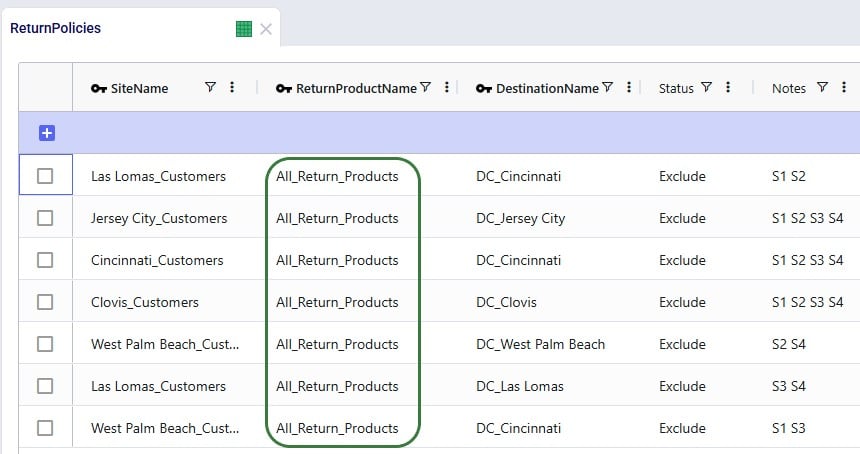
We keep the ratios of how much product comes back for each unit of Bag_1 / Bag_2 sold the same, however we need to update the Return Product Name field on all records to reflect that it is the “_Return” product that comes back. Since this table does not use groups because the return ratios are different for different customer-finished good combinations, the best way to update this table is to also use the bulk update column functionality:
Note that only 4 of the 1,738 records in this table are shown in the screenshot below.
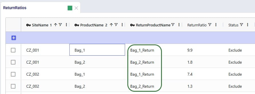
Here, the records representing the lane back from the customers to the DC they send returns back to need to be updated so that the products going back are the “_Return” ones. Since the transportation costs of the return products are the same, we can keep using the grouped policies and just bulk update the Product Name column of the records where Mode Name equals Returns: change the values from the All_Products group to the All_Return_Products group.
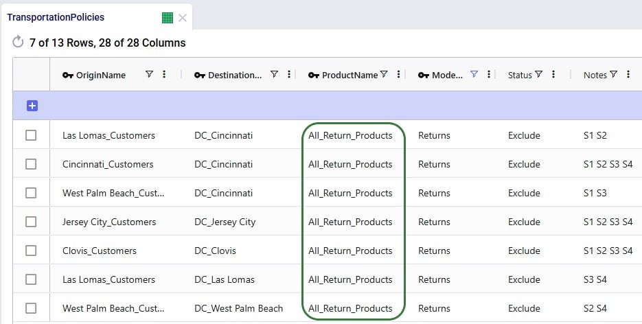
We want to apply the same inbound and outbound handling costs for the return products as we do for the finished goods, so a record is added for the “All_Return_Products” group at All_DCs in the Warehousing Policies table:
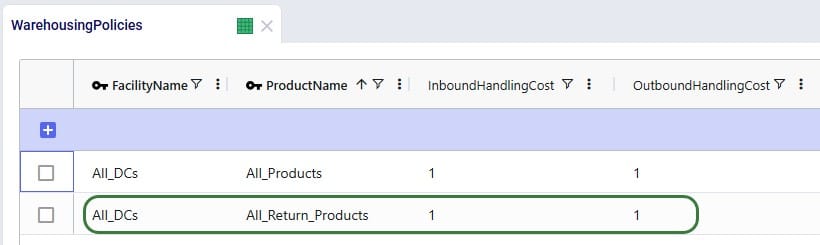
We can use the Bills of Materials (BOM) table to convert the “_Return” products back into the finished goods, applying the desired percentage that will be suitable for reuse. For Bag_1, we want to set up that 70% of the returns can be reused as finished goods, this is done by setting up a BOM as follows (the first 2 records in the screenshot below):
Similarly, we set up the BOM “Reuse_Bag_2” where 1 unit of Bag_2_Return results in 0.5 units of Bag_2 (the 3rd and 4th record in the screenshot):
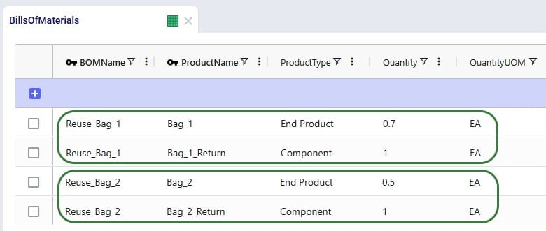
For the BOMs to be used, they need to be associated with the appropriate location-product combinations through production policies. So, we add 2 records to the Production Policies table, which set that at All_DCs the finished goods can be produced using the 2 BOMs. The Unit Cost set on this table represents the cost of inspecting each returned bag and deciding whether it can be reused.
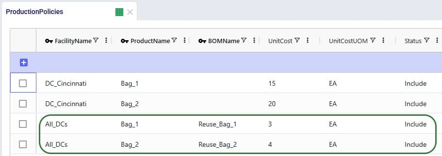
With all the changes made on the input side, we can run the S1 Include Returns scenario (which was copied and renamed to “S1 Include Returns w BOM”). We will briefly look at how these changes affect the outputs.
In the Optimization Return Summary output table, users will notice that the Product Name is still either Bag_1 or Bag_2, but that the Return Product Name is either Bag_1_Return (for Bag_1) or Bag_2_Return (for Bag_2). The quantities are the same as before, since the return ratios are unchanged.

When looking at records of Flow Type = Return, we now see that the Product Name on these flows is that of the “_Return” products.

In this output table, we see that Bag_1 and Bag_2 are no longer only originating from the main DC in Cincinnati, but also at the 2 bigger local DCs that accept returns (Clovis, CA, and Jersey City, NJ) where a percentage of the returns is converted back into sellable finished goods through the BOMs.
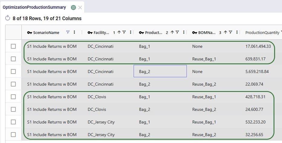
In this appendix we will cover all fields on the 2 new input tables and the 1 new output table.
User-defined variables (UDVs) are a transformative feature in Cosmic Frog’s transportation optimization algorithm (Hopper engine) that allow users to create and track custom metrics specific to their transportation needs. Once established, these variables can be seamlessly integrated into user-defined constraints and/or user-defined costs. Several example use cases are:
Before diving into Hopper’s user-defined variables, costs, and constraints, it is recommended users are familiar with the basics of building and running a Hopper model, see for example this “Getting Started with Hopper” help center article.
In this documentation, we will first describe the example model used to illustrate the UDV concepts in this help article. Next, we will cover the input and output tables available when working with user-defined variables, costs, and constraints. Finally, we will walk through the inputs and outputs of 4 UDV examples: the first two examples showcase the application of constraints to user-defined variables, while the last two examples cover how to model user-defined costs.
The characteristics of the model used to show the concepts of user-defined variables, costs, and constraints throughout this help article are as follows:
The optimized routes from the Baseline_UDV scenario are shown on this map, there are 10 routes with 10 stops each. The customers are color-coded based on the country they are in:
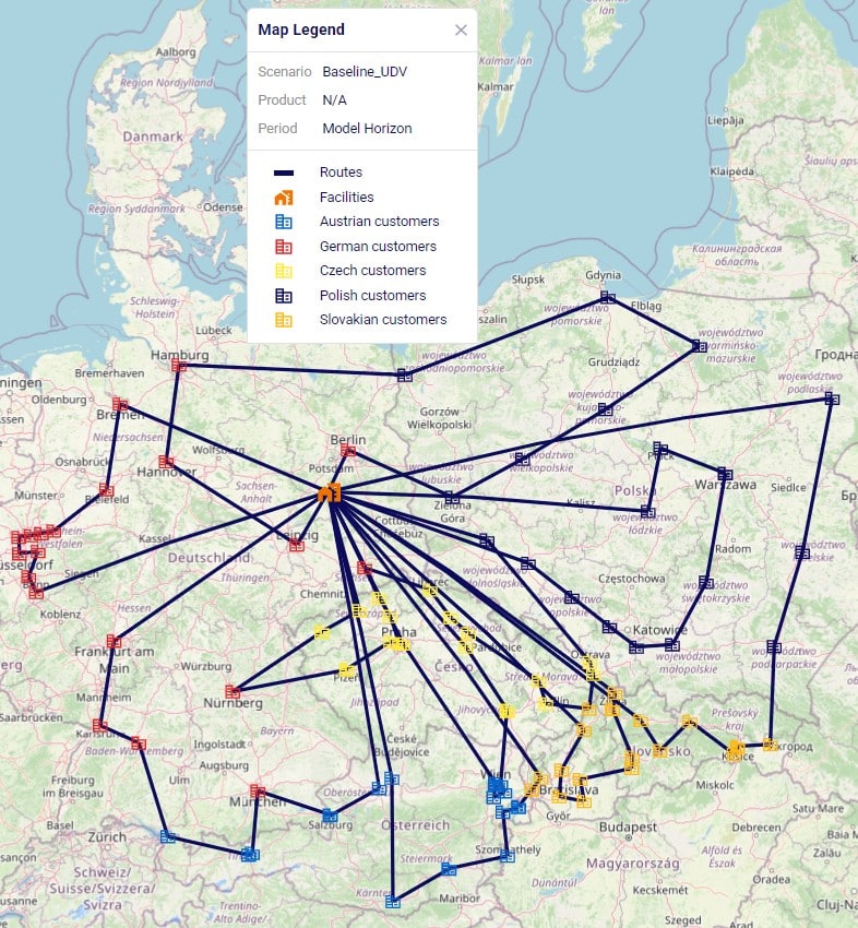
Filtering out the route which has stops in most countries, we find the following route which has stops on it in 4 countries Poland (1 dark blue stop), Czech Republic (7 yellow stops), Slovakia (1 orange stop), and Germany (1 red stop):
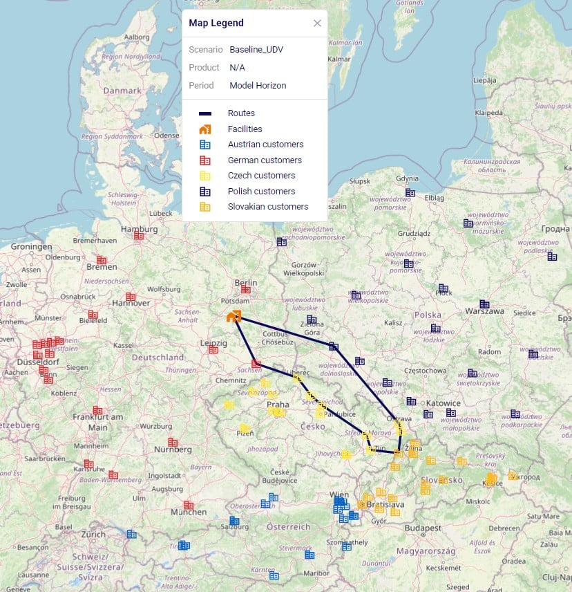
In the Input Tables part of Cosmic Frog’s Data module, there are 3 input tables in the Constraints section that can be used to configure user-defined variables, costs, and constraints:
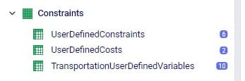
We will take a closer look at each of these input tables now, and will also see more screenshots of these in the later sections that walk through several examples.
On this table we specify the term(s) of each variable which we wish to track or apply user-defined costs and/or constraints to. This first screenshot shows the fields which are used to define the variable, its term(s), and what the return condition is:
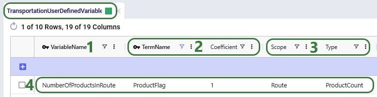
The next 2 screenshots show the other fields available on the Transportation User-Defined Variables input table, which are used to set the Filter Condition for the Scope. Note that several of these fields have accompanying Group Behavior fields, which are not shown in the screenshot. If a group name is used in the Asset Name, Site Name, Shipment ID, or Product Name field, the Group Behavior field specifies how the group should be interpreted: if the Group Behavior field is set to Aggregate (the default if not specified) the activity of the variable is summed over the members of the group, i.e. the variable is applied to the members of the group together. If the Group Behavior field is set to Enumerate, then an instance of the variable will be created for each member of the group individually.


Consider a route which picks up 4 shipments, Shipment #1, #2, #3, and #4, and delivers them to 3 stops on a route as shown in the following diagram. In all 3 examples that follow, the filter condition is set to Shipment ID = Shipment #3 and Site Type = Delivery. This first example shows what will be returned for the variable when Scope = Shipment and Type = Quantity:

The whole route is filtered for Delivery of Shipment #3 and we see that it is delivered to the Delivery 2 stop. Since Scope = Shipment and Type = Quantity, the resulting variable value is the quantity of this shipment, which is what the yellow outline indicates.
In the next example, we look at the same route and same filtering condition (Shipment #3, Delivery), but now Scope has been changed to Stop (Type is still Quantity):
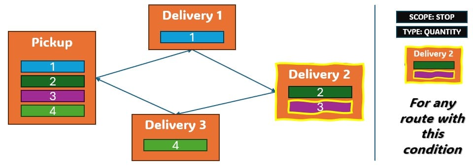
Again, we filter the route for Delivery of Shipment #3 and we see that it is delivered to the Delivery 2 stop. Since Scope = Stop, now the variable value is the total quantity delivered to the stop (outlined in yellow again): quantity Shipment #2 + quantity Shipment #3.
The final visual example is for when the Scope is now changed to Route, while keeping all the other settings the same:
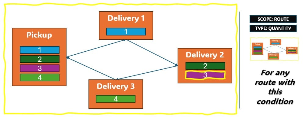
The route is again filtered for Delivery of Shipment #3, since the delivery of this shipment is on this route, we now calculate variable value as the total quantity of the route: quantity Shipment #1 + quantity Shipment #2 + quantity Shipment #3 + quantity Shipment #4, again outlined in yellow.
Next, we will also walk through a numbers example for different combinations of Scope and Type to see how these affect the calculation of the value of a variable’s term. Consider a route with 5 stops as follows:
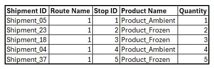
We will calculate the value of the following 15 variables where the Scope, Type, and Product Name to filter for are set to different values. Note that all variables have just 1 term with coefficient 1, so the variable value = scaled term value.
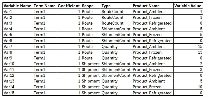
If wanting to apply constraints to user-defined variables, this can be set up on the User-Defined Constraints input table:
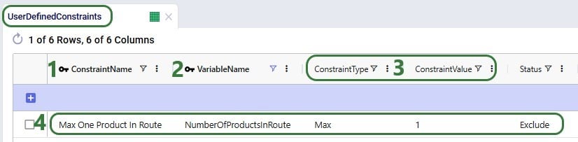
To apply costs to a user-defined variable, this can be achieved by utilizing the User-Defined Costs input table:
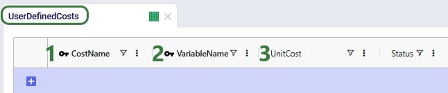
There are 3 output tables related to user-defined costs and constraints:
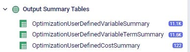
We will cover each of these now and will see more screenshots of them in the sections that follow where we will walk through several example use cases.
This table lists the values of the terms of each user-defined variable. This next screenshot shows the values of the “ProductFlag” term of the “NumberOfProductsInRoute” variable for the routes of the Baseline_UDV scenario. How this variable and its term were set up can be seen in the screenshot of the transportation user-defined variables table above (Scope = Route, Type = Product Count, Coefficient = 1).
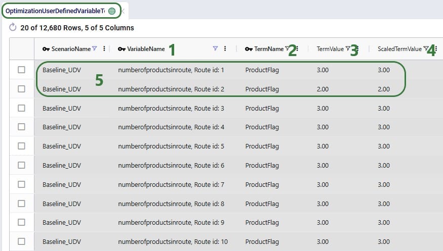
When setting up the Number Of Products In Route variable like above and not applying costs or constraints to it, it functions as a tracker so that user can easily get at this data rather than having to manipulate the transportation optimization output tables to calculate the number of products per route.
If we run a scenario “MaxOneProductPerRoute” where we include the maximum 1 product per route constraint that we have seen in the screenshot in the section further above on the User-Defined Constraints input table, the outputs in this table change as follows:
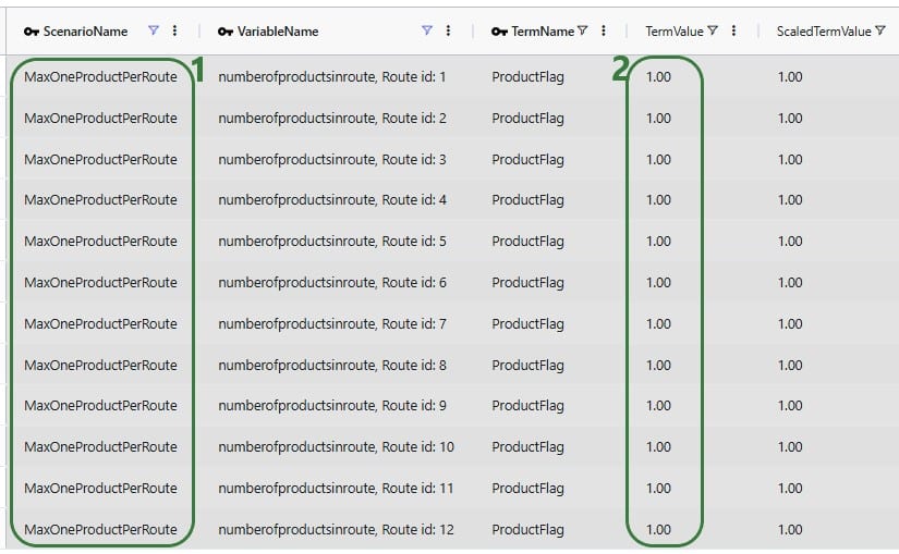
This table is a roll up to the variable level of the Optimization User-Defined Variable Term Summary output table discussed in the previous section. All the scaled terms of each variable have been added up to arrive at the variable’s value:
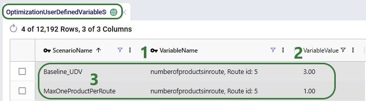
If costs have been applied to a user-defined variable, the results of that can be seen in this output table:

In this first example, we will see how we can track and limit the number of countries per route. For this purpose, a variable with 5 terms is set up in the Transportation User-Defined Variables table. Each term counts if a route has any stops in 1 of the 5 countries used in the model, 1 variable term for each country. Then we will apply constraints to this variable that limit the number of countries on each route to either 1 or 2. Let’s start with looking at the variable and its 5 terms in the Transportation User-Defined Variables table:
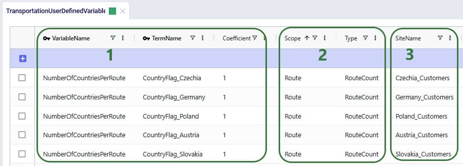
Next, we can add constraints that apply to this variable to change the behavior in the model and limit the number of countries a route is allowed to make stops in on any given route. We use the User-Defined Constraints table for this:
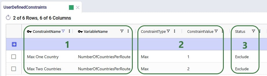
After running the Baseline_UDV scenario which does not include these constraints, we can have a look at the Optimization User-Defined Variable Summary output table:
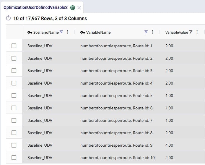
We see that 3 routes make stops in just 1 country, 5 routes in 2 countries, and 1 route (route 9) makes stops in 4 countries when leaving the number of countries a route is allowed to make stops in unconstrained.
Now we want to see the impact of applying the Max One Country and Max Two Countries constraints through 2 scenarios and again we check the Optimization User-Defined Variable Summary output table after running these scenarios:
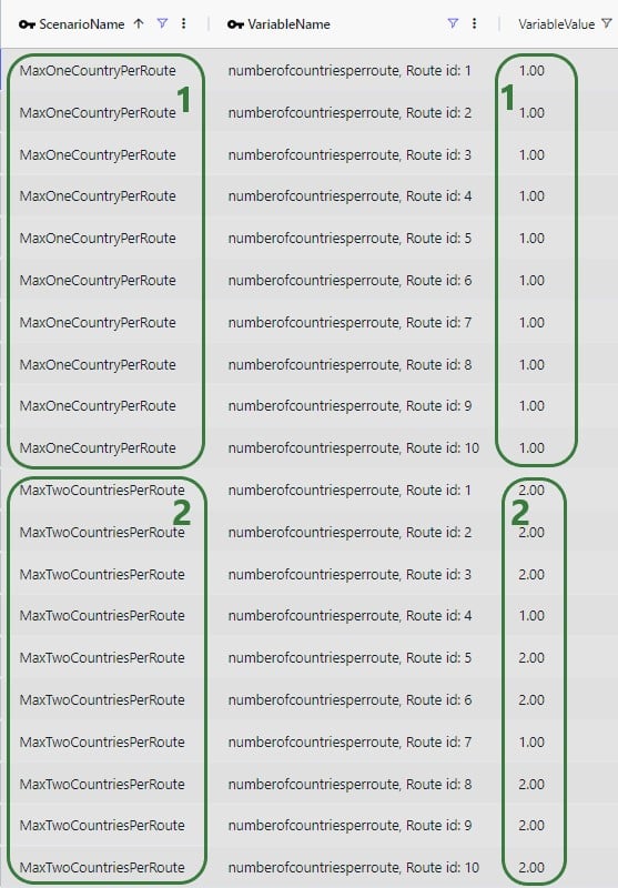
Maps are also helpful to visualize these outputs. As we saw in the introduction of the example model used throughout this documentation, these are the Baseline_UDV routes visualized on a map:
These routes change as follows in the MaxOneCountryPerRoute scenario:

Since some of these routes overlap on the map, let us filter a few out and color-code them based on the country to more easily see that indeed the routes each only make stops in 1 country:
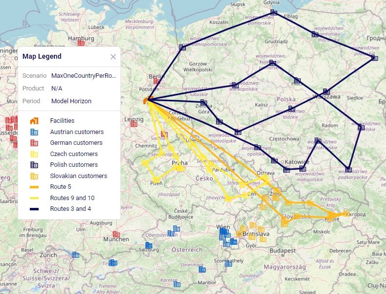
In this example we will see how user-defined variables and constraints can be used to model truck compartments and their capacities. First, we set up 3 variables that track the amount of ambient, refrigerated, and frozen product on a route:
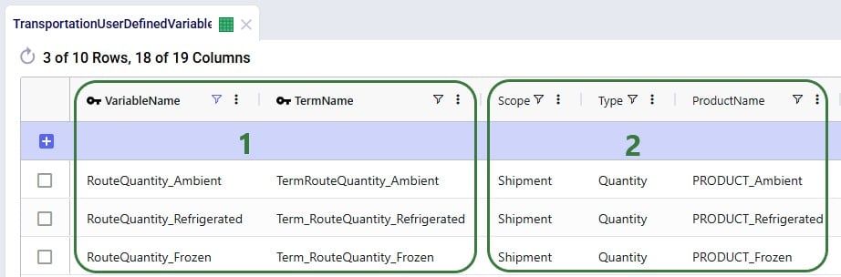
Without setting up any constraints that apply to these variables, they just track how much of each product is on a route, which can be within or over the actual compartment capacity. So, to set capacity limits, we can use the User-Defined Constraints table to setup constraints on these 3 variables that represent the capacity of the ambient, refrigerated, and frozen compartments of a truck:
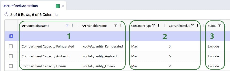
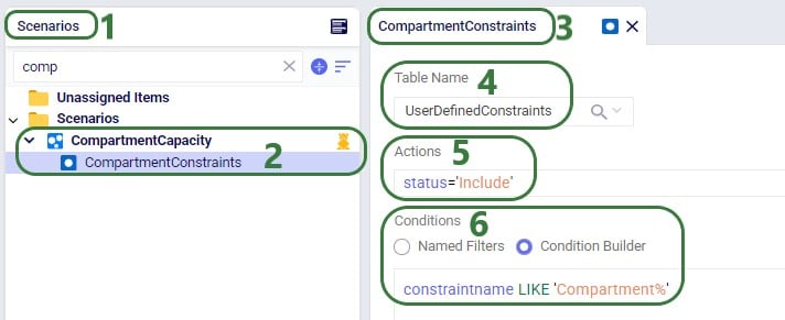
After running the Baseline_UDV scenario where these constraints are not applied and another scenario, Compartment Capacity, where they are applied, we can take a look at the Optimization User-Defined Variable Summary output table to see the effect of the constraints (just showing routes 1 and 2 in the below screenshot):
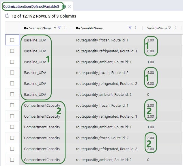
Typically, when adding constraints, we expect routes to change – more routes may be needed to adhere to the constraints, and they may become less efficient. Overall, we would expect costs, distance, and time to increase. This is exactly what we see when comparing these outputs in the Transportation Summary output table for these 2 scenarios:

We have seen 2 examples of applying constraints to user-defined variables in the previous sections. Now, we will walk through 2 examples of applying costs to user-defined variables. The first example shows how to apply a variable cost based on how long a shipment sits on a route: we will specify a cost of $1 per hour the shipment spends on the route. First, we set up a variable that tracks how long a shipment spends on a route in the Transportation User-Defined Variables input table:
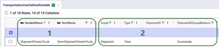
Next, the User-Defined Costs table is used to specify the cost of $1 per hour:
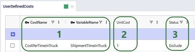
After running the CostPerShipmentTimeInTruck scenario which includes this user-defined cost, we can look at both the Transportation Shipment Summary and the Optimization User-Defined Cost Summary output tables to see this cost of $1 per hour has been applied:
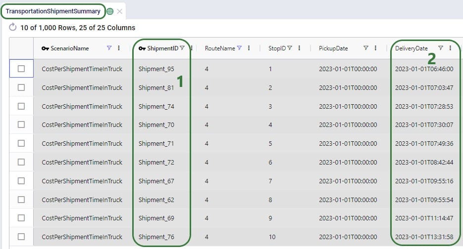
Next, we open the Optimization User-Defined Cost Summary output table and filter for the same scenario and route (#4):
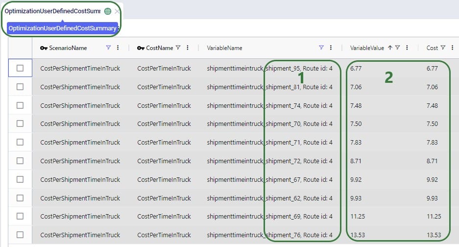
In our final example of this documentation, we will use the same variable ShipmentTimeInTruck from the previous example to set up a different type of cost. We will use it to find any shipments that are on a route for more than 10 hours and apply a penalty cost of $100 to each. This involves using a step cost for which we will also need to utilize the Step Costs table; we will start with looking at this table:
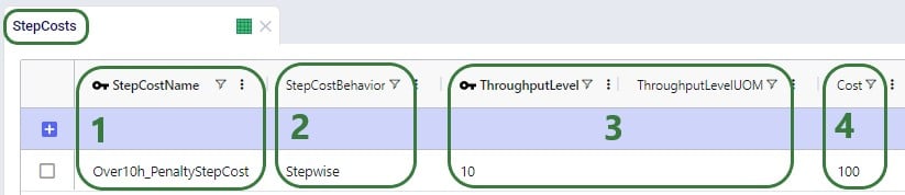
Next, we configure the penalty cost in the User-Defined Costs table:
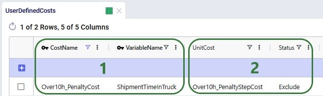
After running a scenario in which we include the penalty cost, we can again look at the Transportation Shipment Summary and Optimization User-Defined Cost Summary output tables to see this cost in action:
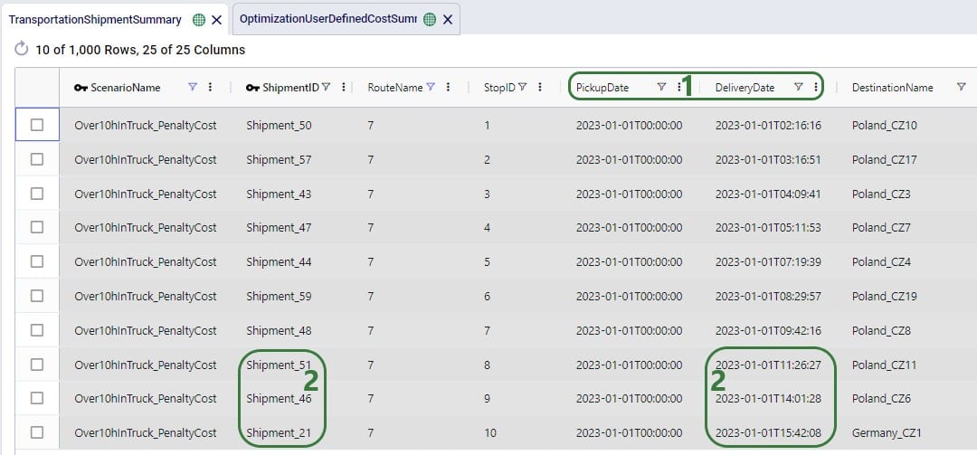
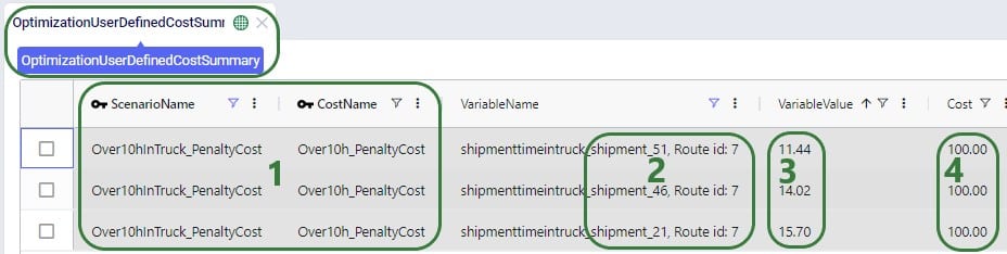
Teams is an exciting new feature set on the Optilogic platform designed to enhance collaboration within Supply Chain Design, enabling companies to foster a more connected and efficient working environment. With Teams, users can join a shared workspace where all team members have seamless access to collective models and files. For a more elaborate introduction to and high-level overview of the Teams feature set, please see this “Getting Started with Optilogic Teams” help center article.
This guide will walk Administrators through the steps to set up their organization and create Teams within the Optilogic platform. For non-administrator users, there is also an “Optilogic Teams – User Guide” help center article available.
To begin, reach out to Optilogic Support at support@optilogic.com and let them know you would like to create your company’s Organization. Once they respond, they will ask you two key questions:
These questions help us determine who should have access to the Organization Dashboard, where organization administrators (“Org Admins”) can manage users, create Teams, invite Members, and more. Specifying your company’s domains also enables us to pre-populate a list of potential users—saving you time by not having to invite each colleague individually.
Once this information is confirmed, our development team will create your organization. When complete, you will be able to log in and begin using the Teams functionality.
If you have been assigned as an Organization Administrator, you can access the Organization Dashboard from the dropdown menu under your username in the top-right corner of the Optilogic platform. Click your name, then select Teams Admin from the list:
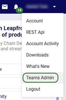
This will take you to your Organization Dashboard, where you can manage Teams and their Members.
We will first look at the Teams application within the Organization Dashboard. Here, all the organization’s teams are listed and can be managed. It will look similar to the following screenshot:


In List View format, the Teams application looks as follows and the same sections of the team edit form mentioned in the above bullets can be opened by clicking on different parts of the team’s record in the list:
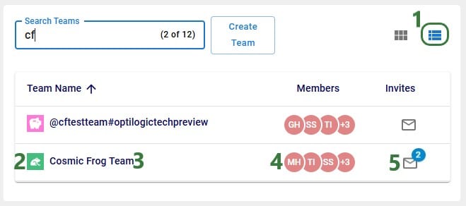
In the Members application, all the organization’s members are listed, and they can be managed here:
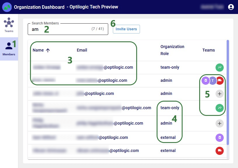
The following diagram gives an overview of the different roles users can have when using Optilogic Teams:
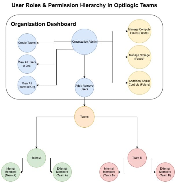
From the Organization Dashboard, while in the Teams application, click the Create Team button (as seen in the screenshots in the “Teams Application for Admins” section above) to start building a new team. The Create New Team form will come up:
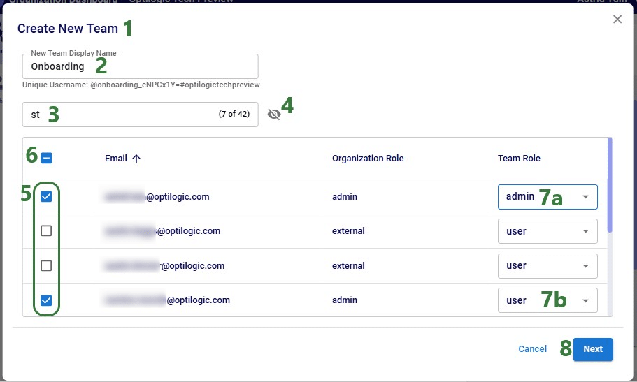
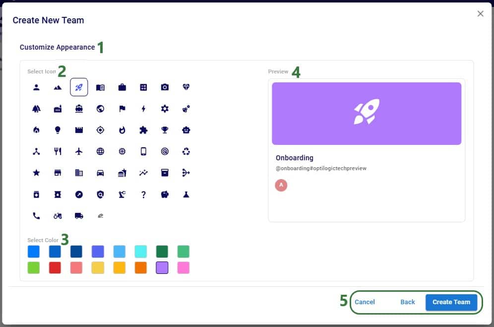
Once a new team is created, members will gain access to the team. If it is their first team, a new application called Team Hub will appear in their list of applications on the Optilogic platform:
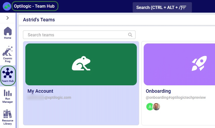
Learn how to use the Team Hub application and about switching between teams and your own My Account in the “Optilogic Teams – User Guide”.
Org Admins can change existing teams by clicking on them in the Teams application while in the Organization Dashboard. Depending on where you click on the team’s card, one of 4 sections of the Edit Team form will be shown, as was also mentioned in the “Teams Application for Org Admins” section further above. When clicking on the name of the Team, the General section is shown:
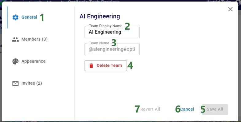
The following screenshot shows the confirmation message that comes up in case an Org Admin clicks on the Delete Team button. If they want to go ahead with the removal of the team, they can click on the Delete button. Otherwise, the Cancel button can be used to not delete the Team at this time.

The second section in the Edit Team form concerns the members of the team:
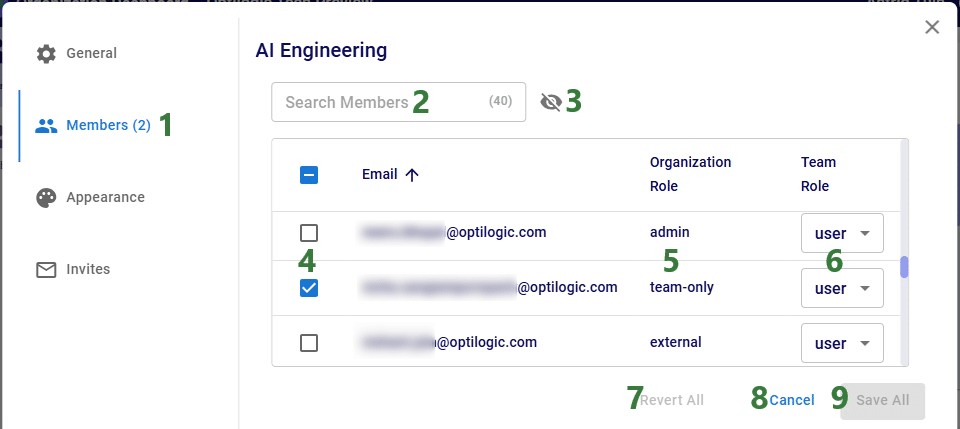
In the third section of the Edit Team form the team’s appearance can be edited:
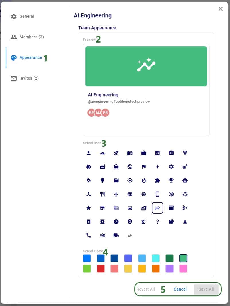
The fourth and last part of the Edit Team form is the Invites section:
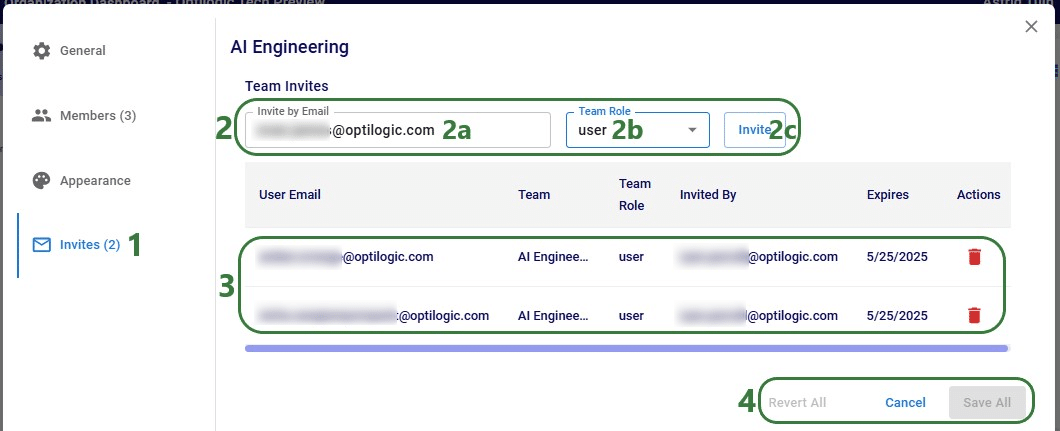
Org Admins can add new users to the organization and/or to teams by clicking on the Invite Users button while in the Members application on the Organization Dashboard. The top part of the form that comes up (next screenshot), will be used to for example add a contractor who will help out your organization for an extended period of time – they become part of the organization and can be added to multiple teams:
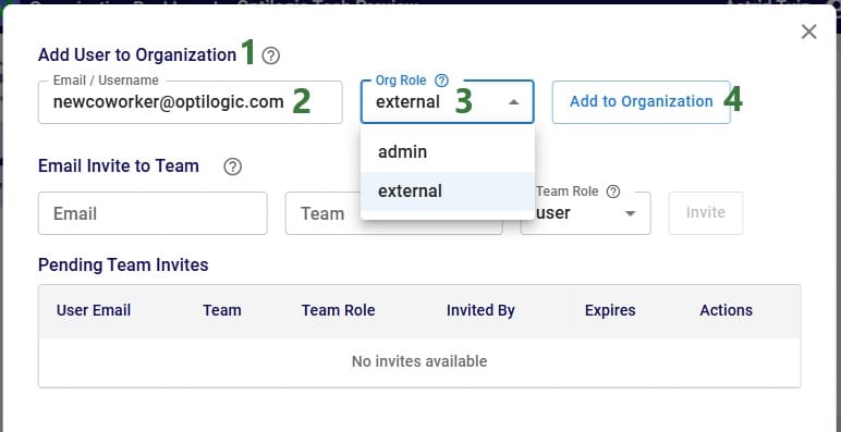
In the second part of this form, people can be invited to a specific team without adding them to the overall organization; these are called Team-only users:
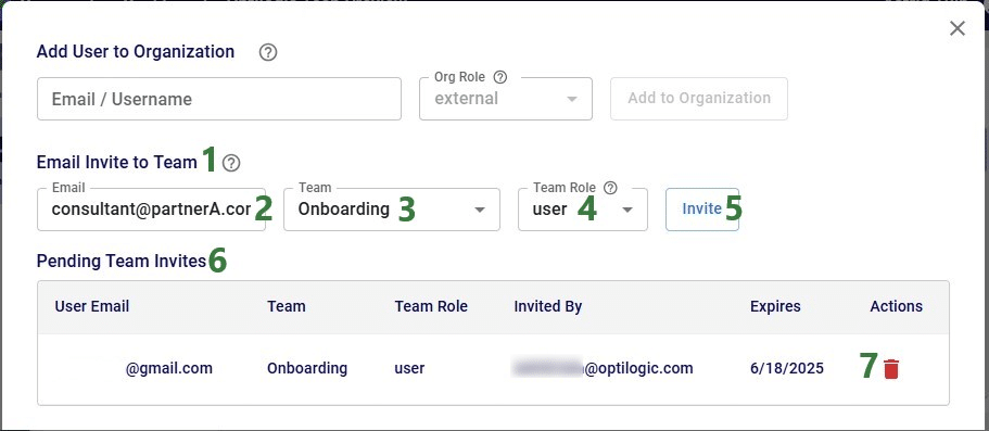

When someone has been emailed an invite to join a team, the email will look similar to the one in the following screenshot:

User can click on the “Click here” link to accept the invite. More on the next steps for a user to join a team can be found in the “Optilogic Teams – User Guide” help center article.
Roles of existing organization members and the teams they are part of can be updated by clicking on the team member in the list of Members:
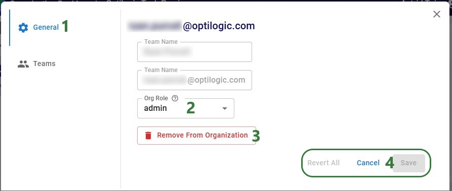

In the Teams section of this form Org Admins can update which team(s) the member is part of and what role they have in those teams:
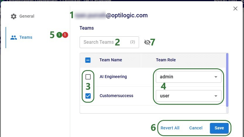
For Team-only members (people who are part of 1 or multiple specific teams, but who are not part of the Organization), a third section named “Invites” will be available on this form:
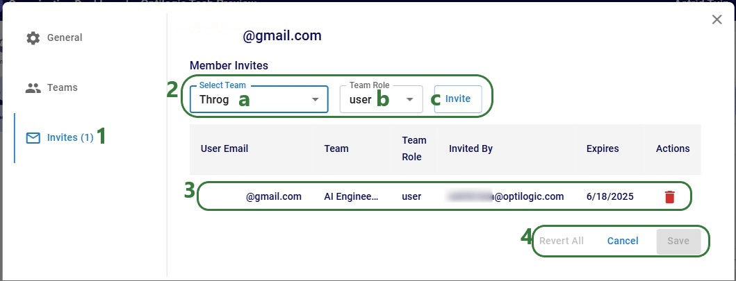
As a best practice, it is recommended to perform regular housekeeping (for example weekly) on your organization’s teams and their members, and your organization’s members. This will prevent situations like a previous employee or temporary consultant still having access to sensitive team contents.
A user with an Org Admin role can also be part of any of the organization’s teams and work inside those or their own My Account workspace. To leave the Organization Dashboard and get back to the Optilogic platform and its applications, they can click on their name at the right top of the organization dashboard and choose “Open Optilogic Platform” from the list:

Here the Admin user can start using the Team Hub application and work collaboratively in teams, the same way as other non-Admin users do. The “Optilogic Teams – User Guide” help center article documents this in more detail.
Once you have set up your teams and added content, you are ready to start collaborating and unlocking the full potential of Teams within Optilogic!
Let us know if you need help along the way—our support team (support@optilogic.com) has your back.
We take data protection seriously. Below is an overview of how backups work within our platform, including what’s included, how often backups occur, and how long they’re kept.
Every backup—whether created automatically or manually—contains a complete snapshot of your database at the time of the backup. This includes everything needed to fully restore your data.
We support two types of backups at the database level:
Often called “snapshots,” “checkpoints,” or “versions” by users:
We use a rolling retention policy that balances data protection with storage efficiency. Here’s how it works:
Retention Tier - Time Period - What’s Retained
Short-Term - Days 1–4 - Always keep the 4 most recent backups
Weekly - Days 5–7 - Keep 1 additional backup
Bi-Weekly - Days 8–14 - Keep the newest and oldest backups
Monthly - Days 15–30 - Keep the newest and oldest backups
Long-Term - Day 31+ - Keep the newest and oldest backups
This approach ensures both recent and historical backups are available, while preventing excessive storage use.
In addition to per-database backups, we also perform server-level backups:
These backups are designed for full-server recovery in extreme scenarios, while database-level backups offer more precise restore options.
To help you get the most from your backup options, we recommend the following:
If you have additional questions about backups or retention policies, please contact our support team at support@optilogic.com.
Teams is an exciting new feature set on the Optilogic platform designed to enhance collaboration within Supply Chain Design, enabling companies to foster a more connected and efficient working environment. With Teams, users can join a shared workspace where all team members have seamless access to collective models and files. For a more elaborate introduction to and high-level overview of the Teams feature set, please see this “Getting Started with Teams” help center article.
This guide will cover how to use and take advantage of the Teams functionality on the Optilogic Platform.
For organization administrators (Org Admins), there is an “Optilogic Teams – Administrator Guide” help center article available. The Admin guide details how Org Admins can create new Teams & change existing ones, and how they can add new Members and update existing ones.
When your organization decides to start using the Teams functionality on the Optilogic platform, they will appoint one or multiple users to be the organizations’s administrators (Org Admin) who will create the Teams and add Members to these teams. Once an Org Admin has added you to a team, you will see a new application called Team Hub when logged in on the Optilogic platform. You will also receive a notification on the Optilogic platform about having been added to a team:
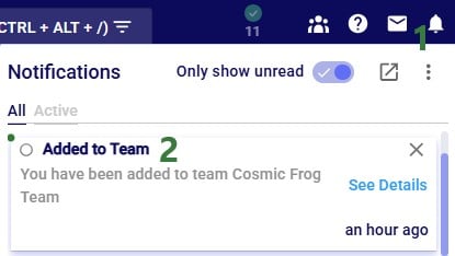
Note that it is possible to invite people from outside an organization to join one of your organization’s teams. Think for example of granting access to a contractor who is temporarily working on a specific project that involves modelling in Cosmic Frog. An Org Admin can invite this person to a specific team, see the “Optilogic Teams – Administrator Guide” help center article on how to do this. If someone is invited to join a team, and they are not part of that organization, they will receive an email invitation to the team. The following screenshots show this from the perspective of the user who is being invited to join a team of an organization they are not part of.
The user will receive an email similar to the one shown below. In this case the user is invited to the “Onboarding” team.
Clicking on the “Click here” link will open a new browser tab where user can confirm to join the team they are invited to by clicking on the Join Team button:
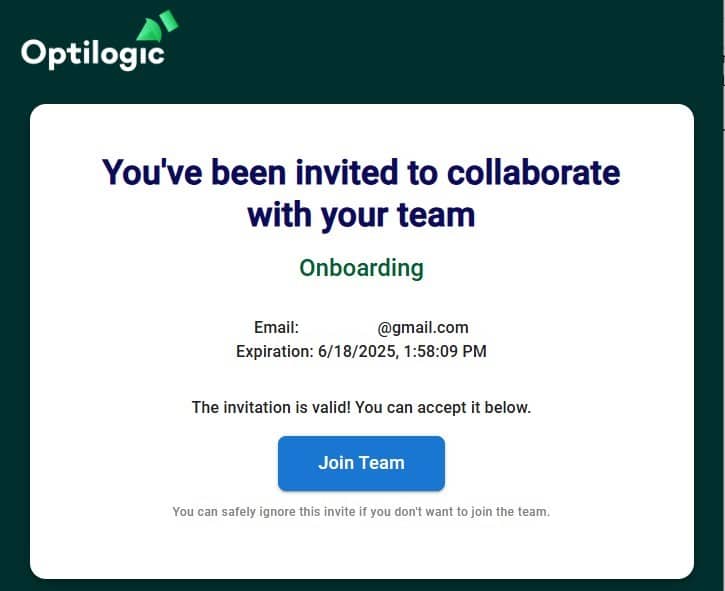
After clicking on the Join Team button, user will be prompted to login to the Optilogic platform or to create an account if they do not have one already. Once logged in, they are part of the team they were invited to and they will see the Team Hub application (see next section).
They will also see a notification in their Optilogic account:

Clicking on the notifications bell icon at the top right of the Optilogic platform will open the notifications list. There will be an entry for the invite the user received to join the Onboarding team.
Should an Org Admin have deleted the invitation before the user accepts the invite, they will get the message “Failed to activate the invite” when clicking on the Join Team button:

The Team Hub is a centralized workspace where users can view and switch between the teams they belong to. At its core, Team Hub provides team members with a streamlined view of their team’s activity, resources, and members. When first opening the Team Hub application, it may look similar to the following screenshot:
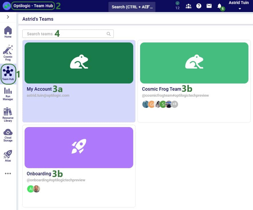
Next, we will have a look at the team card of the Cosmic Frog Team:
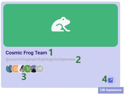

Note that changing the appearance of a team changes it not just for you, but for all members of the team.
When clicking on a team or My Account in the Team Hub, user will be switching into that team and all the content will be that of the team. See also the next section “Content Switching with Team Hub” where this is explained in more detail. When switching between teams or My Account, first the resources of the team you are switching to will be loaded:
Once all resources are loaded, user can click on the Close button at the bottom or wait until it automatically closes after a few seconds. We will first have a look at what the Team Hub looks like for My Account, the user’s personal account, and after that also cover the Team Hub contents of a team.

The overview of a team in the Team Hub application can look similar to following screenshot:
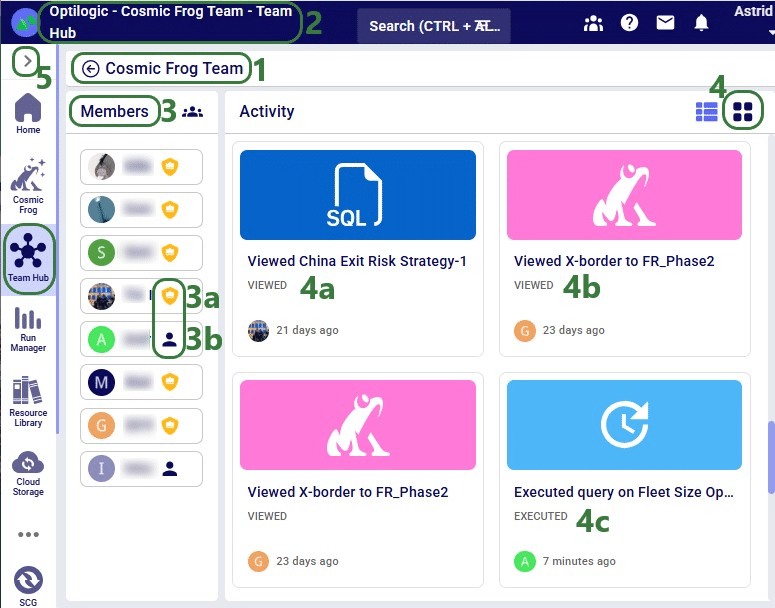
Note that as a best practice, users can start using the team’s activity feed instead of written / verbal updates from team members to understand the details of who worked on what when.
One of the most important features of the Team Hub application is its role as a content switcher. By default, when you log into the Optilogic platform, you’ll see only your personal content (My Account)—similar to a private workspace or OneDrive.
However, once you enter Team Hub and select a specific team, the Explorer automatically updates to display all files and databases associated with that team. This team context extends across the entire Optilogic platform. For example, if you navigate to the Run Manager, you’ll only see job runs associated with the selected team.
By switching into a team, all applications and data within the platform are scoped to that team. We will illustrate this with the following screenshots where user has switched to the team named “Cosmic Frog Team”.
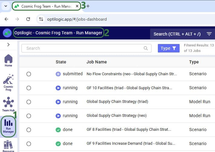
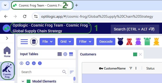
Besides the “Cosmic Frog Team” team, this user is also part of the Onboarding team, which they have now switched to using the Team Hub application. Next, they open Resource Library application:

Note that it is best practice to return to your personal space in My Account when finished working in a Team, to ensure workspace content is kept separate and files are not accidentally created in/added to the wrong team.
Once an organization and its teams are set up, the next step is to start populating your teams with content. Besides adding content by copying from the Resource Library as seen in the last screenshot above, there are two primary ways to add models or files to a team.
Navigate to the Team Hub and switch into your team space. From here, you can create new files, upload existing ones, or begin building new models directly within the team. Keep in mind that any files or models created within a team are visible to all team members and can be modified by them. If you have content that you would prefer not to be accessed or edited by others, we recommend either labeling it clearly or creating it within your personal My Account workspace.

When user is in a specific team (Cosmic Frog Team here), they can add content through the Explorer (expand by clicking on the greater than icon at the top left on the Optilogic Platform): right clicking in the Explorer brings up a context menu with options to create new files, folders, and Cosmic Frog Models, and to upload files. When using these options, these are all created in / added to the active team.
You can also quickly add content to your team by using Enhanced Sharing. This feature allows you to easily select entire teams or individual team members to share content with. When you open the share modal and click into the form, you’ll see intelligent suggestions—teams you belong to and members from your organization—appear automatically. Simply click on the teams or users listed to autofill the form. To learn more about the different ways of sharing content and content ownership, please see the “Model Sharing & Backups for Multi-User Collaboration” help center article.
Please note that, regardless of how a team’s content has been created/added:
Once you have been added to any teams and have added content, you are ready to start collaborating and unlocking the full potential of Teams within Optilogic!
Let us know if you need help along the way—our support team (support@optilogic.com) has your back.
Optilogic introduces the Lumina Tariff Optimizer – a powerful optimization engine that empowers companies to reoptimize supply chains in real-time to reduce the effects of tariffs. It provides instant clarity on today’s evolving tariff landscape, uncovers supply chain impacts, and recommends actions to stay ahead – now and into the future.
Manufacturers, distributors, and retailers around the world are faced with an enormous task trying to keep up with changing tariff policies and their supply chain impact. With Optilogic’s Lumina Tariff Optimizer, companies can illuminate their path forward by proactively designing tariff mitigation strategies that automatically consider the latest tariff rates.
With Lumina Tariff Optimizer, Optilogic users can stay ahead of tariff policy and answer critical questions to take swift action:
The following 7-minute video gives a great overview of the Lumina Tariff Optimizer tools:
Optilogic’s Lumina Tariff Optimization engine can be leveraged by modelers within Cosmic Frog or be leveraged within a Cosmic Frog for Excel app for other stakeholders across the business to evaluate the tariff impact to their end-to-end supply chain. Optilogic enables users to get started quickly with Lumina with several items in the Resource Library that include:
This documentation will cover each of these Lumina Tariff Optimizer tools, in the same order as listed above.
The first tool in the Lumina Tariff Optimizer toolset is the Tariffs example model which users can copy to their own account from the Resource Library. We will walk through this model, covering inputs and outputs, with emphasis on how to specify tariffs and their impact on the optimal solution when running network optimization (using the Neo engine) on the scenarios in the model.
Let us start by looking at the map of the Tariffs model, which is showing the model locations and flows for the Baseline scenario:
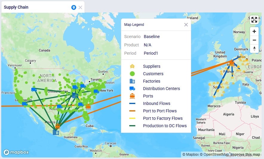
This model consists of the following sites:
Next, we will have a look at the Products table:

As mentioned above, raw materials RM1, RM2, and RM3 are supplied by Chinese suppliers and the others 6 raw materials by European suppliers, which we can confirm by looking at the Supplier Capabilities input table:
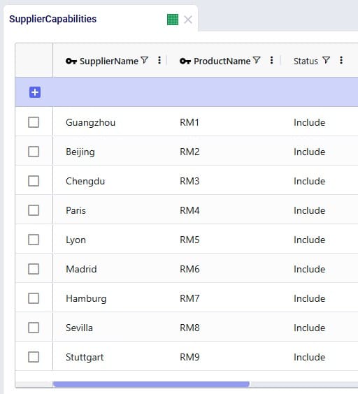
The Bills Of Materials input table shows that each finished good takes 3 of the Raw Materials to be manufactured; the Quantity field indicates how much of each is needed to create 1 unit of finished good:

Looking at the Production Policies input table, we see that both the US and Mexico factory can produce Consumables, but Rockets are only manufactured in Mexico and Space Suits only in the US:
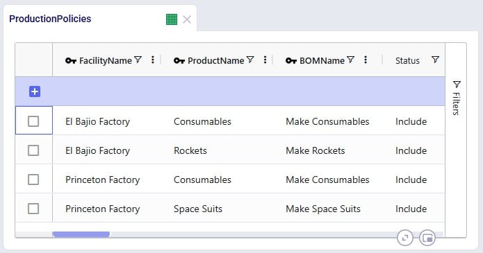
To understand the outputs later, we also need to briefly cover the Flow Constraints input table, which shows that the El Bajio Factory in Mexico can at a maximum ship out 3.5M units of finished goods (over all products and the model horizon together):

To enter tariffs and take them into account in a network optimization (Neo) run, users need to populate the new Tariffs input table:
There are also 2 new Neo output tables that will be populated when tariffs are included in the model, the Optimization Path Flow Summary and the Optimization Tariff Summary tables:
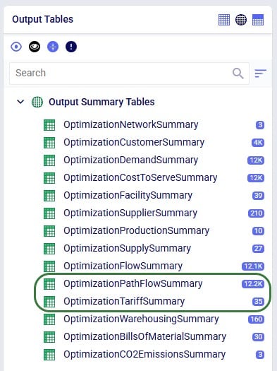
Tariffs can be specified at multiple levels in Cosmic Frog, so users can choose the one that fits their modeling needs and available data best:
In order to model tariffs from/to a region or country, these fields need to be populated in the Customers, Facilities, and Suppliers tables:

In the Tariffs input table, all path origin location (furthest upstream) – path destination location (furthest downstream) – product combinations to which tariffs need to be applied are captured. There can be any number of echelons in between the path origin location and path destination location where the product flows through. Consider the following path that a raw material takes:

The raw material is manufactured/supplied from China (the path origin), it then flows through a location in Vietnam, then through a location in Mexico, before ending its path in the USA (the path destination, where it is consumed when manufacturing a finished good). In this case the tariff that is set up for this raw material with path origin = China, and path destination = USA will be applied. The tariff will be applied to the segment of the path where the product arrives in the region / country of its final destination. In the example here, that is on last leg (/lane / segment) of the path, e.g. on the Mexico to USA lane.
If we have a raw material that takes the same initial path, except it ends in Mexico to be consumed in a finished good, then the tariff that is set up for this raw material with path origin = China and path destination = Mexico will be applied. To continue from this example: then if this finished good manufactured in Mexico is shipped to the US and sold there, and if there is a path with a tariff set up from Mexico to USA for the finished good, then that tariff will be applied (path origin = Mexico, path destination = USA). I.e. in this last example the entire path is just the 1 segment between Mexico and USA.
So, now we will look how this can be set up in the Tariffs input table:
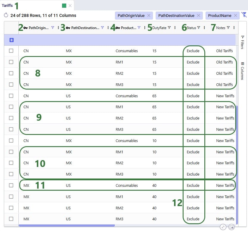
Please note:
Three scenarios were run in the Tariffs example model:
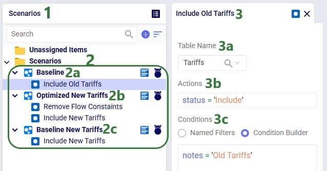
Now, we will look at the outputs for these 3 scenarios, first at a higher level and later on, we will dig into some details of how the tariff costs are calculated as well.
The Financials stacked bar chart in the standard Optimization Scenario Comparison dashboard in the Analytics module of Cosmic Frog can be used to compare all costs for all 3 scenarios in 1 graph:
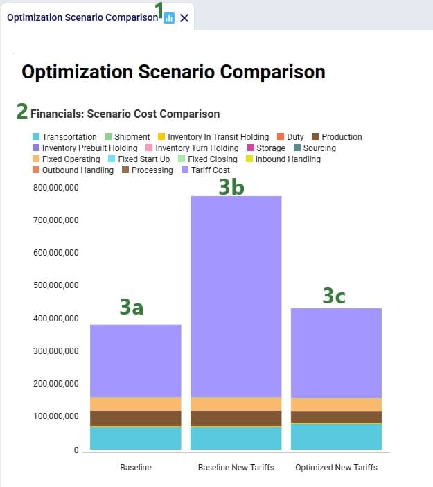
To compare the Tariffs by path origin – path destination and product, a new “Optimization Tariffs Summary” dashboard was created. We will look at the Baseline New Tariffs scenario first, and the Optimized New Tariffs scenario next:
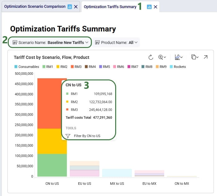
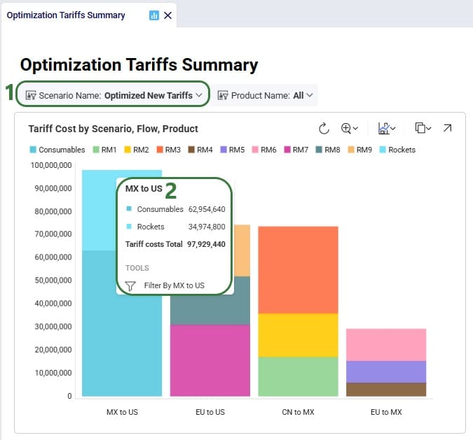
Note that in the Appendix it is explained how this chart can be created.
Next, we will take a closer look at some more detailed outputs. Starting with how much demand there is in the model for Rockets and Consumables, the 2 finished goods the Mexican factory in El Bajio can manufacture. The next screenshot shows the Optimization Demand Summary network optimization output table, filtered for Rockets and with a summation aggregation applied to it to show the total demand for Rockets at the bottom of the grid:
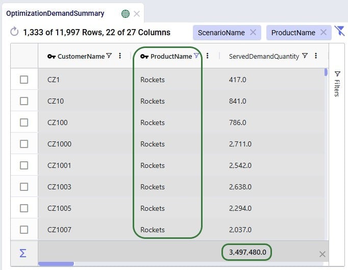
Next, we change the filter to look at the Consumables product:

In conclusion: the demand for Rockets is nearly 3.5M units and for Consumables nearly 10.5M. Rockets can only be produced in Mexico whereas Consumables can be produced by both factories. From the charts above we suspected a shift in production from US to Mexico for the Consumables finished good in the Optimized New Tariffs scenario, which we can confirm by looking at the Optimization Production Summary output table:
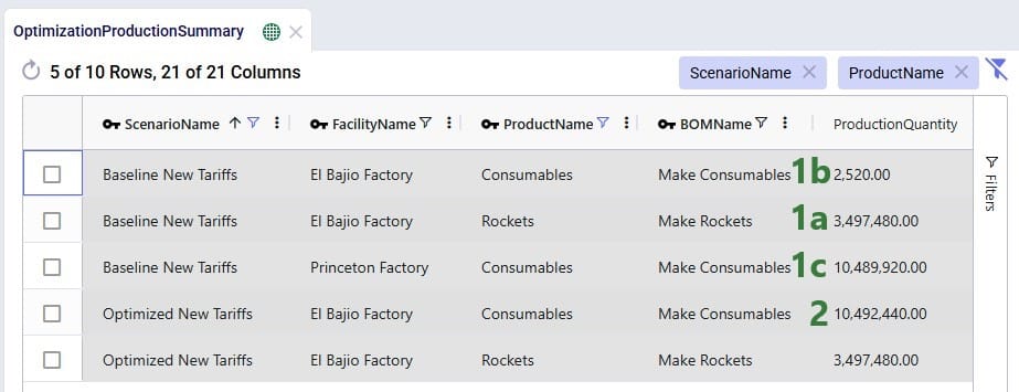
Since the production of Consumables requires raw materials RM1, RM2, and RM3, we expect to see the above production quantities for Consumables to be reflected in the amount of these raw materials that was moved from the suppliers in China to the US vs to Mexico. We can see this in the Optimization Flow Summary network optimization output table, which is filtered for the 2 scenarios with new tariffs, Port to Port lanes, and these 3 raw materials:

The custom Optimization Tariff Summary and Optimization Path Flow Summary output tables are automatically generated after running a network optimization on a model with a populated Tariffs table. The first of these 2 is shown in the next screenshot where we have filtered out the raw materials RM1, RM2, and RM3 again, plus also the Consumables finished good for the 2 scenarios that use the new tariffs:

Where the Optimization Tariff Summary output table summarizes the tariffs at the scenario - path origin – path destination – product level, the Optimization Path Flow Summary output table gives some more detail around the whole path, and on which segments the tariffs are applied. The next 2 screenshots show 6 records of this output table for the Tariffs example model:
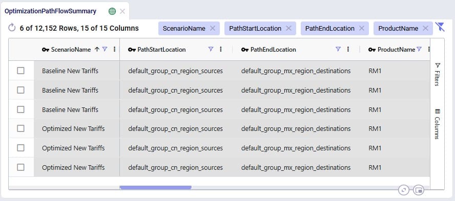
For the 2 scenarios that use the new tariffs, records are filtered out for raw material RM1 where the Path Start Location represents the CN region and the Path End Location represents the MX region. These Path Start and End Locations are automatically generated based on the Path Origin Property and Value and Destination Property and Value set in the Tariffs input table. Scrolling right for these 6 records:
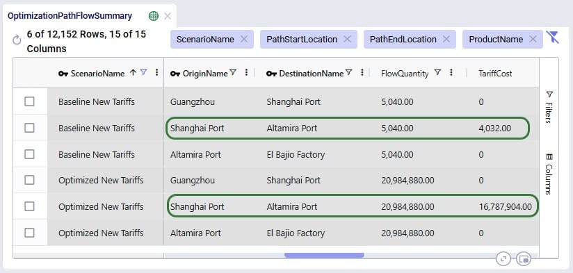
We see that the path for RM1 is the same in both scenarios: originate at location Guangzhou in China, moved to Shanghai Port (CN), from Shanghai Port moved to Altamira Port (MX), and from Altamira Port moved to the El Bajio Factory (MX). The calculations of the Tariff Cost based on the Flow Quantity are the same as explained above, and we see that the tariffs are applied on the second segment where the product arrives in the region / country of its final destination.
Wondering where to go from here? If you are wanting to start using tariffs in your own models, but are not exactly sure where to start, please see the “Cosmic Frog Utilities to Create the Tariffs Table” section further below, which also includes step-by-step instructions based on what data you have available.
In the next section, we will first discuss how quick sensitivity analyses around tariffs can be run using a Cosmic Frog for Excel App.
To enable Cosmic Frog users, and also managers and executives with no or limited knowledge of Cosmic Frog, to run quick sensitivity scenarios around changing tariffs, Optilogic has developed an Excel Application for this specific purpose. Users can connect to their Cosmic Frog model that contains a populated Tariffs input table and indicate which tariffs to increase/decrease by how much, run network optimization with these changed tariffs, and review the optimization tariff summary output table, all in 1 Excel workbook. Users can download this application and related files from the Resource Library.
The following represents a typical workflow when using the Tariffs Rapid Optimizer application:
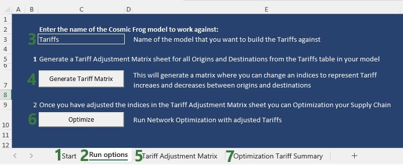

For users to take advantage of the power of the Lumina Tariff Optimizer they will want to create their own network optimization model which includes a populated Tariffs input table (see also the “Tariffs Model – Tariffs Table” section earlier in this documentation). Depending on the data available to the user, populating the Tariffs input table can be a straightforward task or a difficult one in case no or little data around tariffs is known/available within the organization. Optilogic has developed 3 utilities to help users with this task. The utilities are available from within Cosmic Frog, which will be covered in this section of the documentation, and they are also available through the Cosmic Frog for Excel Tariffs Builder App, which will be covered in the next section. Here follows a short description of each utility, they will each be covered in more detail later in this section:
In Cosmic Frog, they are accessible from the Utilities module (click on the 3 horizontal bars icon at the top left in Cosmic Frog to open the Module menu drop-down and select Utilities):
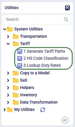
The utilities are listed under System Utilities > Tariff.
The latter 2 utilities hook into Avalara APIs, and users need to use / obtain their own Avalara API keys for each to be able to use these utilities from within Cosmic Frog or the Tariffs Builder Excel App.
The following list shows the recommended steps for users with varying levels of Tariffs data available to them from least to most data available (assuming an otherwise complete Cosmic Frog model has been built):
To populate the Tariffs table with all possible path origin – path destination – product combinations, based on the contents of the Transportation Policies input table, use this first utility:
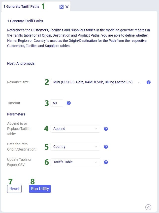
Consider a small model with 1 customer in the US, 2 facilities (1 DC and 1 factory) both in the US, 1 supplier in China, and 2 products (1 finished good and 1 component):
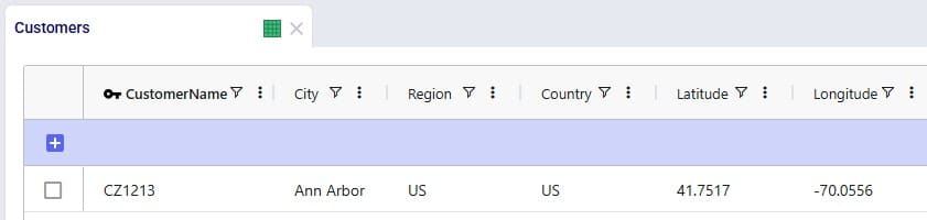
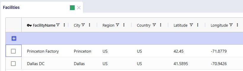
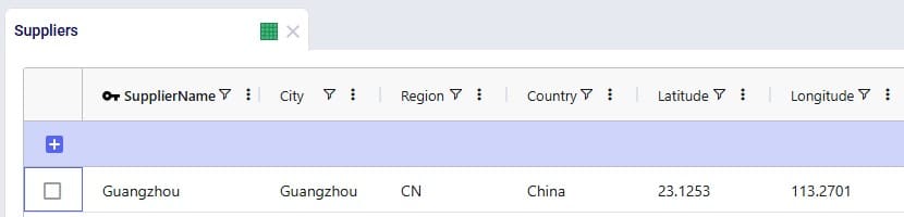
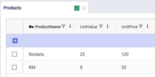
After running the 1 Generate Tariff Paths utility (using Region as the data to use for the path origin and path destination), the Tariffs table is generated and populated as shown in the next 2 screenshots:
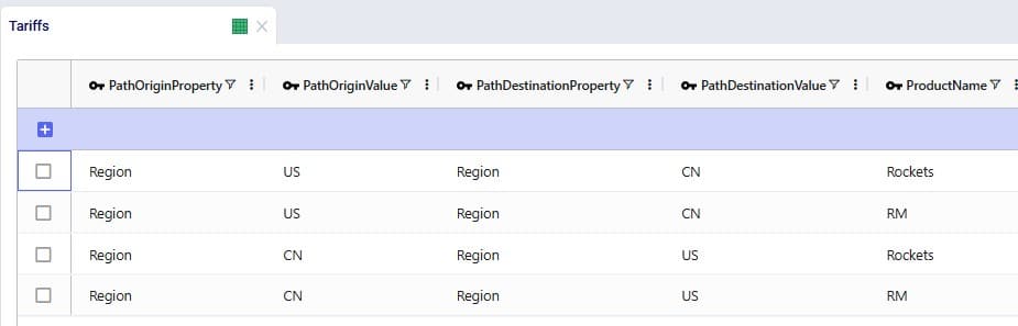
All combinations for path origin region, path destination region, and product have been added to the Tariffs table. Scrolling further right, we see the remaining fields of this table:
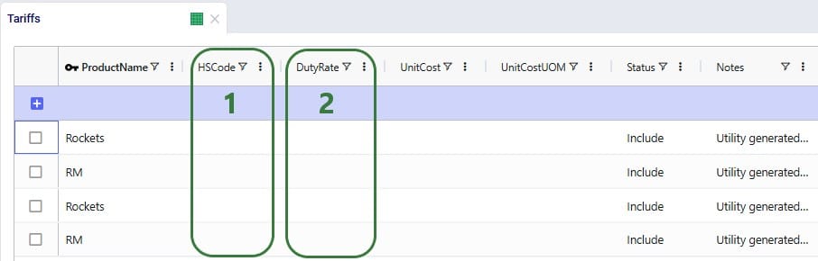
To update the HS Code field in the Tariffs table, we can use the second utility:
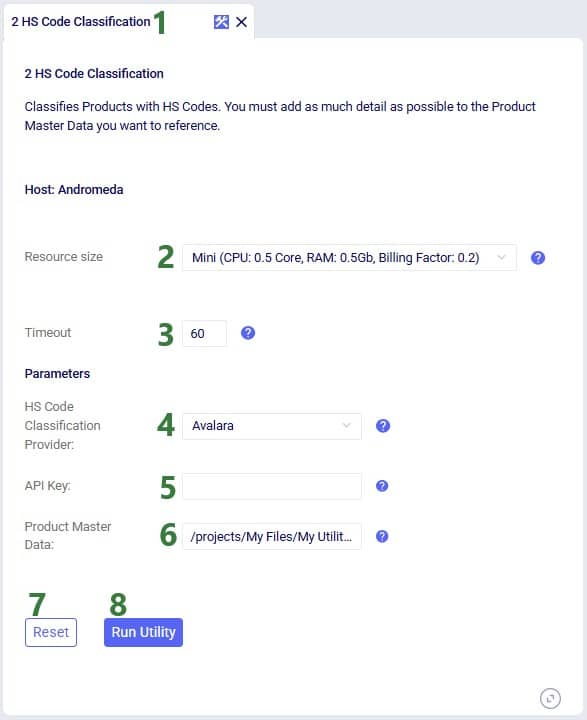
Users can find the full path of a file uploaded to their Optilogic account as follows:
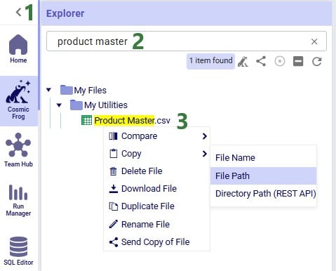
The file containing the product master data needs to have the same columns as shown in the next screenshot:
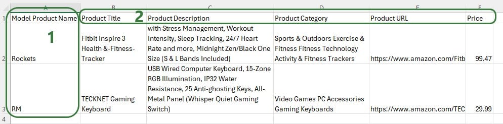
Note that columns B-F contain information of products that do not match the product name in Cosmic Frog as this is just an example to show how the utility works.
After running the 2 HS Code Classification utility, we see that the HS Code field in the Tariffs table is now populated:
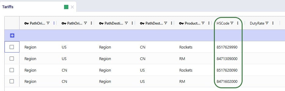
To use the HS Code field to next look up duty rates we can use the third utility:
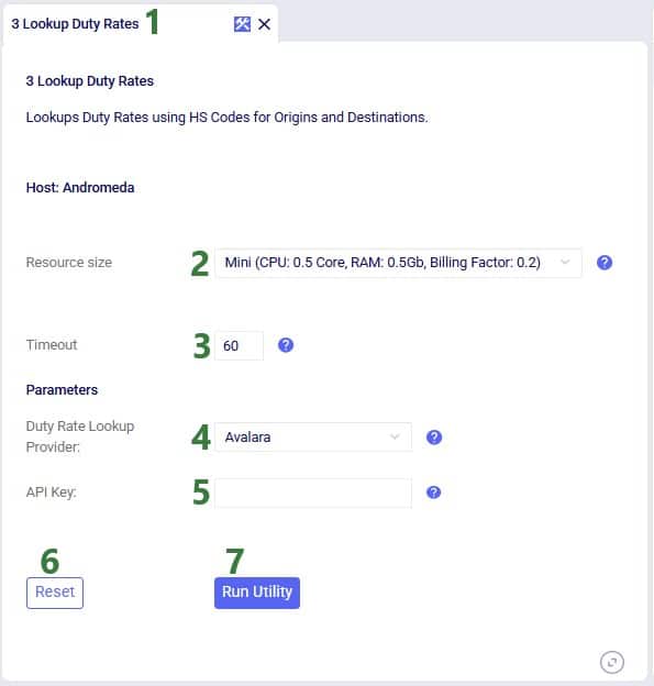
After running the 3 Lookup Duty Rates utility, we see that the Duty Rate field in the Tariffs table is now populated:
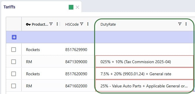
The raw output from the API is placed in the Duty Rate field and user needs to update this so that the field contains just a number representing the total duty rate. For the second record (US region to China region for product RM), the total duty rate is 35% (25% + 10%), and user needs to enter 35 in this field. For the third record (China region to US region for product Rockets), the duty rate is 27.5% (7.5% + 20%), and user needs to enter 27.5 in this field. For the fourth record (China region to US region for product RM), the total duty rate is 25%, and user needs to enter 25 in this field.
When running a utility in Cosmic Frog, user can track the progress in the Model Activity window:
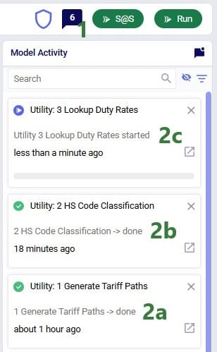
The 3 utilities covered in the previous section to generate and populate the Tariffs input table are also made available in the Cosmic Frog for Excel Tariffs Builder App, which we will cover in this section. Users can download this application and related files from the Resource Library.
The following represents a typical workflow when using this Tariffs Builder application:
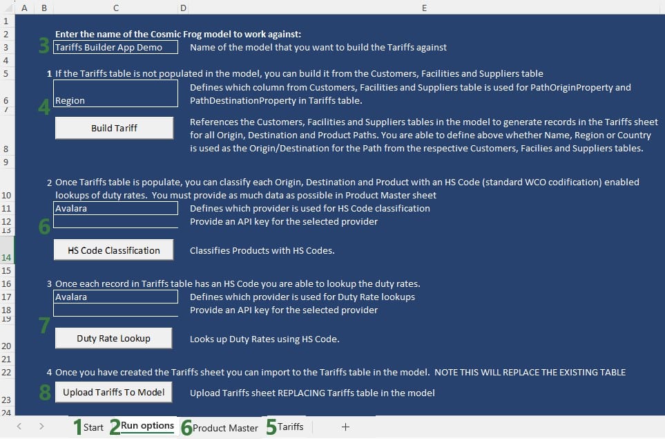
The next screenshot shows the Tariffs table after just running the Build Tariff workflow (bullet 4 in the list above):
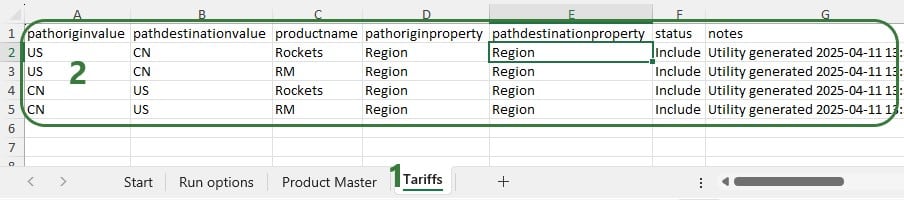
The next screenshot shows the Product Master worksheet which contains the product information to be used by the HS Code Classification workflow, it needs to be in this format and users should enter as much product information in here as possible:
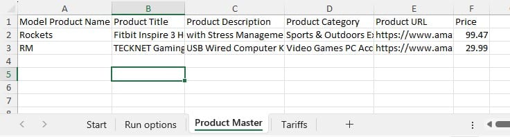
After also running the HS Code Classification and the Duty Rate Lookup workflows (bullets 6 and 7 in the list further above), we see that these fields are now also populated on the Tariffs worksheet:
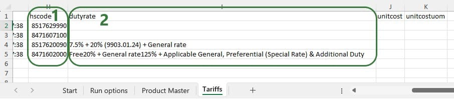
We hope users feel empowered to take on the challenging task of incorporating tariffs into their optimization workflows. For any questions, please do not hesitate to contact Optilogic support on support@optilogic.com.
In this appendix we will show users how to create a stacked bar chart for each path origin – path destination pair, showing the tariff costs by product.
In the Analytics drop-down menu in the toolbar while in the Analytics module of Cosmic Frog, select New Dashboard, give it a name (e.g. Optimization Tariff Summary), then click on the blue Visualization button on the top right to create a new chart for the dashboard. In the New Visualization configuration form that comes up, type “tariff” in the Tables Search box, then check the box for the Optimization Tariff Summary table in the list, and click on Select Data.
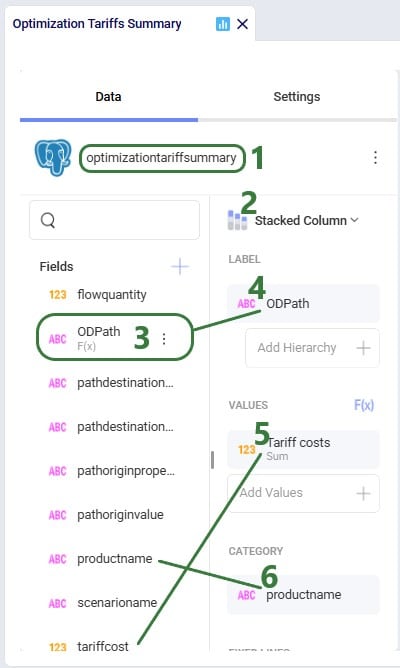
To create the OD Path calculated field, click on the plus icon at the top right of the Fields list and select Calculated Field which brings up the Edit Calculated Field configuration window:
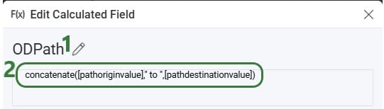
Tax systems can be complex, like for example those in Greece, Colombia, Italy, Turkey, and Brazil are considered to be among the most complex ones. It can however be important to include taxes, whether as a cost or benefit or both, in supply chain modeling as they can have a big impact on sourcing decisions and therefore overall costs. Here we will showcase an example of how Cosmic Frog’s User Defined Variables and User Defined Costs can be used to model Brazilian ICMS tax benefits and take these into account when optimizing a supply chain.
The model that is covered in this documentation is the “Brazil Tax Model Example” which was put together by Optilogic’s partner 7D Analytics. It can be downloaded from the the Resource Library. Besides the Cosmic Frog model, the Resource Library content also links to this “Cosmic Frog – BR Tax Model Video” which was also put together by 7D Analytics.
A helpful additional resource for those unfamiliar with Cosmic Frog’s user defined variables, costs, and constraints is this “How to use user defined variables” help article.
In this documentation the setup of the example model will first be briefly explained. Next, the ICMS tax in Brazil will be discussed at a high level, including a simplified example calculation. In the third section, we will cover how ICMS tax benefits can be modelled in Cosmic Frog. And finally, we will look at the impact of including these ICMS tax benefits on the flows and overall network costs.
One quick note upfront is that the screenshots of Cosmic Frog tables used throughout this help article may look different when comparing to the same model in user’s account after taking it from the Resource Library. This is due to columns having been moved or hidden and grids being filtered/sorted in specific ways to show only the most relevant information in these screenshots.
In this example model, 2 products are included: Prod_National to represent products that are made within Brazil at the MK_PousoAlegre_MG factory and Prod_Imported to represent products that are imported, which is supplied from SUP_Itajai_SC within the model, representing the seaport where imported products would arrive. There are 6 customer locations which are in the biggest cities in Brazil; their names start with CLI_. There are also 3 distribution centers (DCs): DC_Barueri_SP, DC_Contagem_MG, and DC_FeiraDeSantana_BA. Note that the 2 letter postfixes in the location names are the abbreviations of the states these locations are in. Please see the next screenshot where all model locations are shown on a map of Brazil:
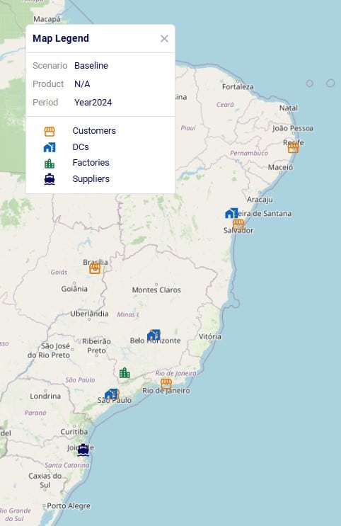
The model’s horizon is all of 2024 and the 6 customers each have demand for both products, ranging from 100 to 600 units. The SUP_ location (for Prod_Imported) and MK_ location (for Prod_National) replenish the DCs with the products. Between the DCs, some transfers are allowed too. The demand at the customer locations can be fulfilled by 1, 2 or all 3 DCs, depending on the customer. The next screenshot of the Transportation Policies table (filtered for Prod_National) shows which procurement, replenishment, and customer fulfillment flows are allowed:
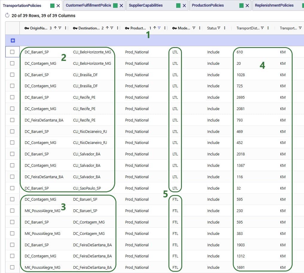
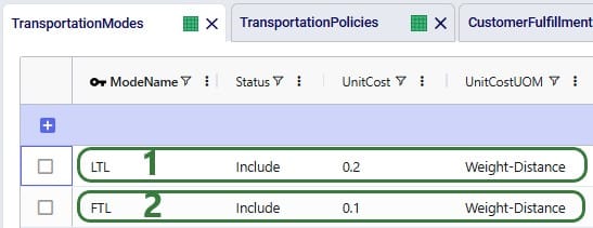
For the other product modelled, Prod_Imported, the same customer fulfillment, DC-DC transfer, and supply options are available, except:
In Brazil, the ICMS tax (Imposto sobre Circulaçao de Mercadorias e Serviços, or Tax on Commerce and Services) is levied by the states. It applies to movement of goods, transportation services between several states or municipalities, and telecommunication services. The rate varies and depends on the state and product.
When a company sells a product, the sales price includes ICMS, which results in an ICMS debit for the company (the company owes this to the state). Likewise, when purchasing or transferring product, the ICMS is included in what the company pays the supplier. This creates ICMS credit for the company. The difference between the ICMS debits and credits is what the company will pay as ICMS tax.
The next diagram shows an ICMS tax calculation example, where company also has a 55% tax benefit which is a discount on the ICMS it needs to pay.
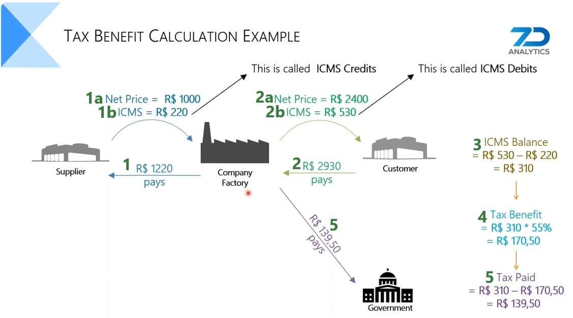
In order to include ICMS tax benefits in a model, we need to be able to calculate ICMS debits and credits based on the amount of flow between locations in different states for both national and imported products. As different states and different products can have different ICMS rates, we need to define these individual flow lanes as variables and apply the appropriate rate to each. This can be done by utilizing the User Defined Variables and User Defined Costs input tables, which can be found in the “Constraints” section of the Cosmic Frog input tables, shown in the below screenshot (here user entered a search term of “userdef” to filter out these 2 tables):
In the User Defined Variables table, we will define 3 variables related to DC_Contagem_MG: one that represents the ICMS Debits, one that represents the ICMS Credits, and one that represents the ICMS Balance (= ICMS Debits – ICMS Credits) for this DC. The ICMS Debits and ICMS Credits variables have multiple terms that each represents a flow out of or a flow into the Contagem DC, respectively. Let us first look at the ICMS Debits variable:
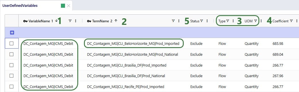
Still looking at the same top records that define the DC_Contagem_MG|ICMS_Debit variable, but freezing the Variable Name and Term Name columns and scrolling right, we can see more of the columns in the User Defined Variables table:
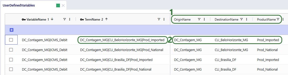
Note that there are quite a few custom columns in this table (not shown in the screenshots; can be added through Grid > Table > Create Custom Column), which were used to calculate the ICMS rates outside of the model. These are helpful to keep in the model, should changes need to be made to the calculations.
Next, we will have a look at the ICMS Credit variable, which is made up of 3 terms, where each term represents a possible supply/replenishment flow into the Contagem DC:
The last step on the User Defined Variables table is to combine the ICMS Credit and ICMS Debit variables to calculate the ICMS balance:
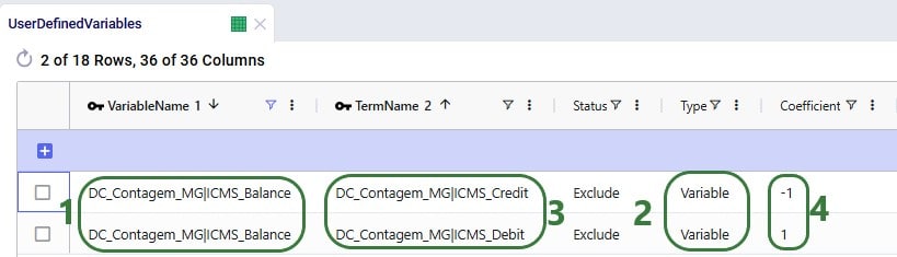
To finalize the setup, we need to add 1 record to the User Defined Costs table, where we will specify that the company has a 55% discount (tax incentive) for the ICMS it pays relating to the Contagem DC:

As mentioned in the previous section, all records in the User Defined Variables and User Defined Costs tables have their Status set to Exclude. This way, when the Baseline scenario is run, the ICMS tax incentive is not included, and the network will be optimized just based on the costs included in the model (in this case only transportation costs). We want to include the ICMS tax incentive in a scenario and then compare the outputs with the Baseline scenario. This “IncludeDCMGTaxBenefit” scenario is set up as follows:
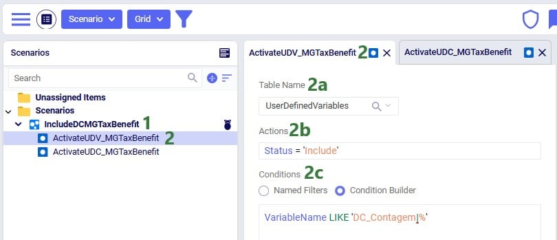
Next, we have a look at the second scenario item that is part of this scenario:

With the scenario set up, we run a network optimization (using the Neo engine) on both scenarios and then first look in the Optimization Network Summary output table:
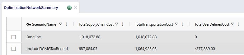
Notice that the Baseline scenario as expected only contains transportation costs, while the IncludeDCMGTaxBenefits scenario also contains user defined costs, which represent the calculated ICMS tax benefit and have a negative value. So, overall, the IncludeDCMGTaxBenefit scenario has about R$ 331k lower total cost as compared to the Baseline scenario, even though the transportation costs are close to R$ 47k higher. Since the transportation costs are different between the 2 scenarios, we expect some of the flows have changed.
There are 3 network optimization output tables that contain the outputs related to User Defined Variables and Costs:

We will first discuss the Optimization User Defined Variable Term Summary output table:
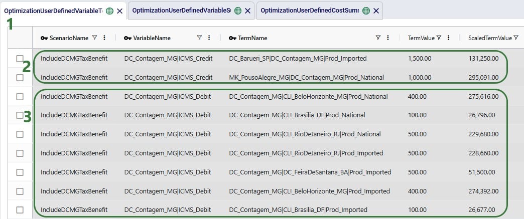
The Optimization User Defined Variable Summary output table contains the outputs at the variable level (e.g. the individual terms of the variables have been aggregated):
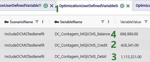
Finally, the Optimization User Defined Cost Summary output table shows the cost based on the 55% benefit that was set:

The DC_Contagem_MG_TaxIncentive benefit is calculated from the DC_Contagem_MG|ICMS_Balance variable, where the Variable Value of R$ 686,980 is multiplied by -0.55 to arrive at the Cost value of R$ -377,839.
Now that we understand at a high level the cost impact of the ICMS tax incentive and the details of how this was calculated, let us look at more granular outputs, starting with looking at the flows between locations. Navigate to the Maps module within Cosmic Frog and open the maps named Baseline and Include DC MG Tax Benefit, which show outputs from the Baseline and IncludeDCMGTaxBenefit scenarios, respectively. The next 2 screenshots show the flows from DCs to customer locations: Baseline flows in the top screenshot and scenario “Include DC MG Tax Benefit” flows in the bottom screenshot:
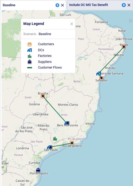
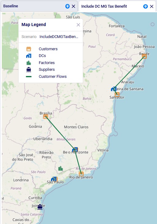
We see that in the Baseline the customer in Rio de Janeiro is served by the DC in Sao Paulo. This changes in the scenario where the tax benefit is included: now the Rio de Janeiro customer is served by the Contagem DC (located close to Belo Horizonte). The other customer fulfillment flows are the same between the 2 scenarios.
This model also has 2 custom dashboards set up in the Analytics module; the 1. Scenarios Overview dashboard contains 2 graphs:

This Summary graph shows the cost buckets for each scenario as a bar chart. As discussed when looking at the Optimization Network Summary output table, the IncludeDCMGTaxBenefit scenario has an overall lower cost due to the tax benefit, which offsets the increased transportation costs as compared to the Baseline scenario.
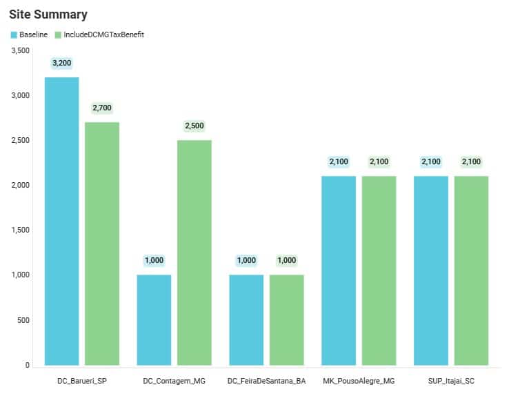
This Site Summary bar chart shows the total outbound quantity for each DC / Factory / Supplier by scenario. We see that the outbound flow for the DC in Barueri is reduced by 500 units in the IncludeDCMGTaxBenefit scenario as compared to the Baseline scenario, whereas the Contagem DC has an increased outbound flow, from 1,000 to 2,500 units. We can examine these shifts in further detail in the second custom dashboard named 2. Outbound Flows by Site, as shown in the next 2 screenshots:

This first screenshot of the dashboard shows the amount of flow from the 3 DCs and the factory to the 6 customer locations. As we already noticed on the map, the only shift here is that the Rio De Janeiro customer is served by the Barueri DC in the Baseline scenario and this changes to it being served by the Contagem DC in the IncludeDCMGTaxBenefit scenario.

Scrolling further right in this table, we see the replenishment flows from the 3 DCs and the Factory to the 3 DCs. There are some more changes here where we see that the flow from the factory to the Barueri DC is reduced by 500 units in the scenario, whereas the flow from the factory to the Contagem DC is increased by 500 units. In the Baseline, the Barueri DC transferred a total of 1,000 units to the other 2 DCs (500 each to the Contagem and Feira de Santana DCs), and the other 2 DCs did not make DC transfers. In the Tax Benefit scenario, the Barueri DC only transfers to the Contagem DC, but now for 1,500 units. We also see that the Contagem DC now transfers 500 units to the Feira de Santana DC, whereas it did not make any transfers in the Baseline scenario.
We hope this gives you a good idea of how taxes and tax incentives can be considered in Cosmic Frog models. Give it a go and let us know of any feedback and/or questions!
Leapfrog helps Cosmic Frog users explore and use their model data via natural language. View data, make changes, create & run scenarios, analyze outputs, learn all about the Anura schema that underlies Cosmic Frog models, and a whole lot more!
Leapfrog combines an extensive knowledge of PostgreSQL with the complete knowledge of Optilogic’s Anura data schema, and all the natural language capabilities of today’s advanced general purpose LLMs.
For a high-level overview and short video introducing Leapfrog, please see the Leapfrog landing page on Optilogic’s website.
In this documentation, we will first get users oriented on where to find Leapfrog and how to interact with it. In the section after, Leapfrog’s capabilities will be listed out with examples of each. Next, the Tips & Tricks section will give users helpful pointers so they can get the most out of Leapfrog. Finally, we will step through the process of building, running, and analyzing a Cosmic Frog model start to finish by only using Leapfrog!
Dive in if you’re ready to take the leap!
Start using Leapfrog by opening the module within Cosmic Frog:
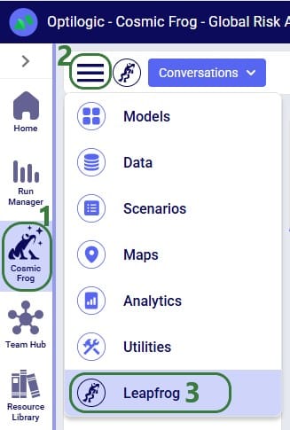
Once the Leapfrog module is open, users’ screens will look similar to the following screenshot:
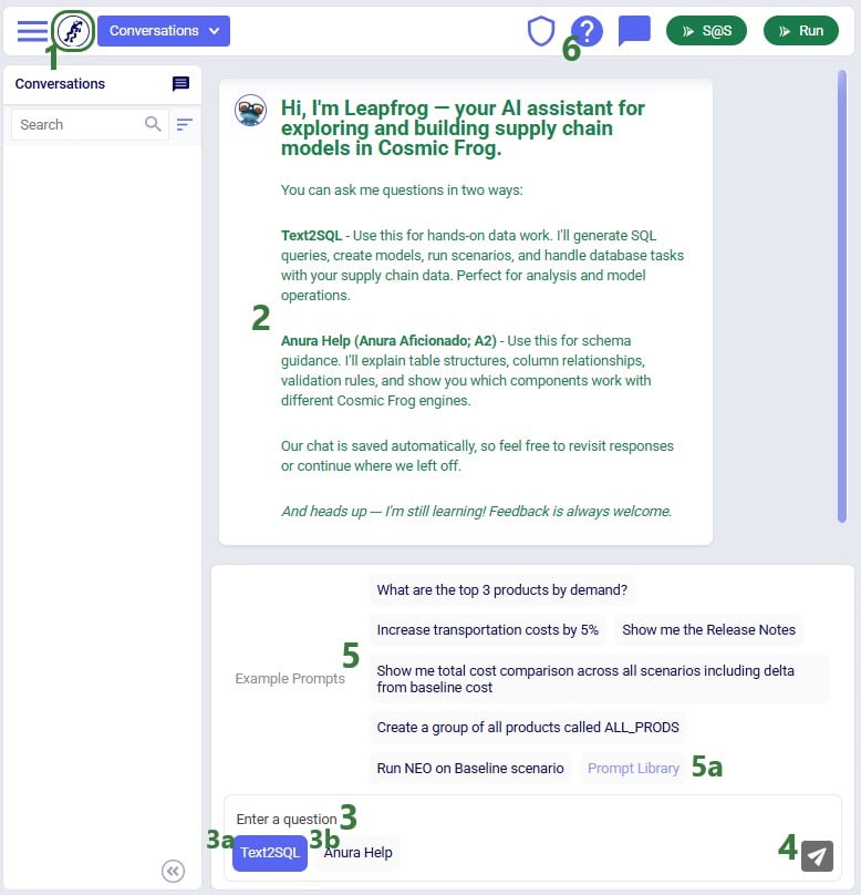
The example prompts when using the Anura Help LLM are shown here:
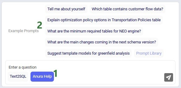
When first starting to use Leapfrog, users will also see the Privacy and Data Security statement, which reads as follows:
“Leapfrog AI Training: Optilogic does not use your model data to train Leapfrog. We do collect and store conversational data so it can be accessed again by the user, as well as to understand usage patterns and areas of strength/weakness for the LLM. Included in this data: natural language input prompts, text and SQL responses, as well as feedback from users. This information is maintained by Optilogic, not shared with third parties, and all of the conversation data is subject to the data security and privacy terms of the Optilogic platform.”

This message will stay visible within Leapfrog whenever it is being used, unless user clicks on the grey cross button on the right to close the message. Once closed, the message will not be shown again while using Leapfrog.
Conversation history is stored on the platform at the user level - not in the model database - so it does not get shared when a model is shared. Note that if you are working in a Team rather than in your My Account (see documentation on Teams on the Optilogic platform here), the Leapfrog conversations you are creating will be available to the other team members when they are working with the same model.
As mentioned in the previous section, Leapfrog currently makes use of 2 large language models (LLMs): Text2SQL and Anura Help (also referred to as Anura Aficionado or A2). They will be explained in some more detail here. There is also an appendix to this documentation where for a few example personas Leapfrog questions and responses are listed, which showcases how some users may predominantly use one model, while others may switch back and forth between them. Of course, when unsure, users can try a specific prompt using both LLMs to see which provides the most helpful response.
Please note that in future users will not need to indicate which LLM they want to run a prompt against as Leapfrog will recognize which one will be most suitable to use based on the prompt.
The Text2SQL LLM combines extensive knowledge of PostgreSQL with Optilogic’s Anura data schema, and all the natural language capabilities of today’s advanced general purpose LLMs. It has been further fine-tuned on a large set of prompt-response pairs hand-crafted by supply chain modeling experts. This allows the Text2SQL model to generate SQL queries from natural language prompts.
Prompts for which it is best to use the Text2SQL model often imply an action: “Show me X”, “Add Y”, “Delete Z”, “Run scenario A”, “Create B”, etc. See also the example prompts listed when starting a new conversation and those in the Prompt Library on the Frogger Pond community.
Leapfrog responses using this model are usually actionable: run the returned SQL query to add / edit / delete data, create a scenario or model, run a scenario, geocode locations, etc.
A full list of the capabilities of both LLMs is covered in the section “Leapfrog Capabilities” further below.
Anura Help (also referred to as Anura Aficionado or A2) is a specialized assistant that leverages advanced natural language processing to help users navigate and understand the Anura schema within Optilogic's Cosmic Frog application. The Anura schema is the foundational framework powering Cosmic Frog's optimization, simulation, and risk assessment capabilities. Anura Help eliminates traditional barriers to schema understanding by providing immediate, authoritative guidance for supply chain modelers, developers, and analysts.
Anura Help’s architecture uses the Retrieval Augmented Generation (RAG) approach: based on the natural language prompt, first the most relevant documents of those in its knowledge base are retrieved (e.g. schema details or engine awareness details). Next, it uses them to generate a natural language response.
Use the Anura Help model when wanting to learn about specific fields, tables or engines in Cosmic Frog. Its core capabilities include:
Responses from Leapfrog when using the Anura Help model are text-based and generated from retrieved documents shown in the context section. This context can for example be of the category “column info” where all details for a specific field are listed.
A full list of the capabilities of both LLMs is covered in the section “Leapfrog Capabilities” further below.
The following list compares the 2 LLMs available in Leapfrog today:
Depending on the type of question, Leapfrog’s response to it can take different forms: text, links, SQL queries, data grids, and options to create models, scenarios, scenario items, groups, run scenarios, or geocode locations. We will look at several examples of questions that result in these different types of responses in this section. This is not an exhaustive list; the next section “Leapfrog Capabilities” will go through the types of prompt-response pairs Leapfrog is capable of today.
For our first question, we used the first Text2SQL example prompt “What are the top 3 products by demand?” by clicking on it. After submitting the prompt, we see that Leapfrog is busy formulating a response:
And Leapfrog’s response to the prompt is as follows:
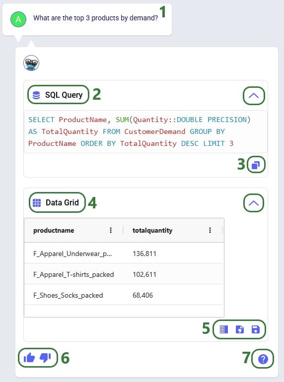
The metadata included here are:
Clicking on the icon with 3 dots again will collapse the response metadata.
This first prompt asked a question about the input data contained in the Cosmic Frog model. Let us now look at a slightly different type of prompt, which asks to change model input:
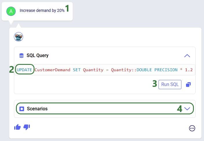
We are going to run the SQL query of the above response to our “Increase demand by 20%” prompt. Before doing so, let’s review a subset of 10 records of the Customer Demand input table (under the Data Module, in the Input Tables section):
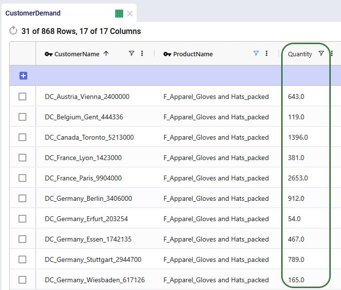
Next, we will run the SQL query:
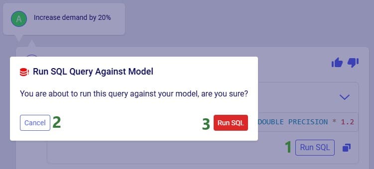
After clicking the Run SQL button at the bottom of the SQL Query section in Leapfrog’s response, it becomes greyed out so it will not accidentally be run again. Hovering over the button also shows text indicating the query was already run:
Note that closing and reopening the model or refreshing the browser will revert the Run SQL button’s state so it is clickable again.
Opening the Customer Demand table again and looking at the same 10 records, we see that the Quantity field has indeed been changed to its previous value multiplied by 1.2 (the first record’s value was 643, and 643 * 1.2 = 771.6, etc.):
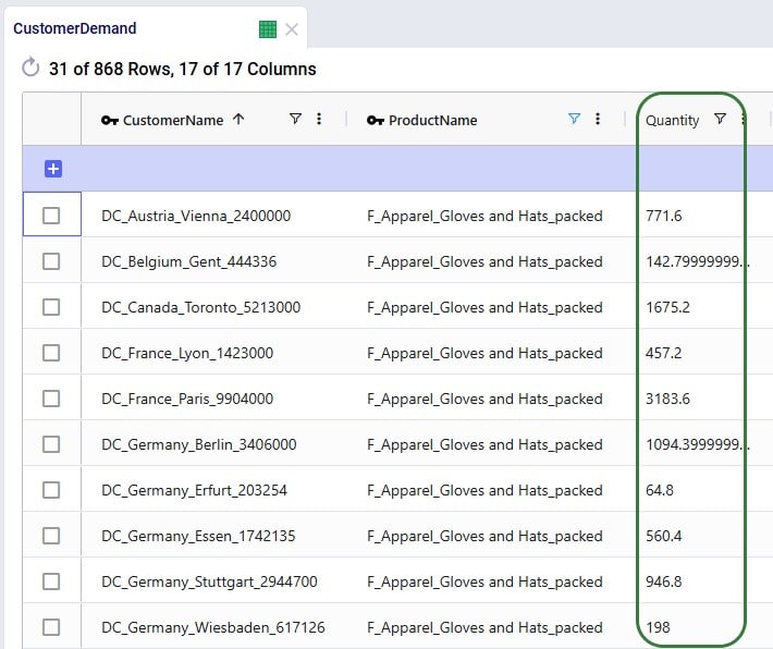
Running the SQL query to increase the demand by 20% directly in the master data worked fine as we just saw. However, if we do not want to change the master data, but rather want to increase the demand quantity as part of a scenario, this is possible too:
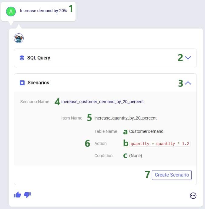
After navigating to the Scenarios module within our Cosmic Frog model, we can see the scenario and its item have been created:
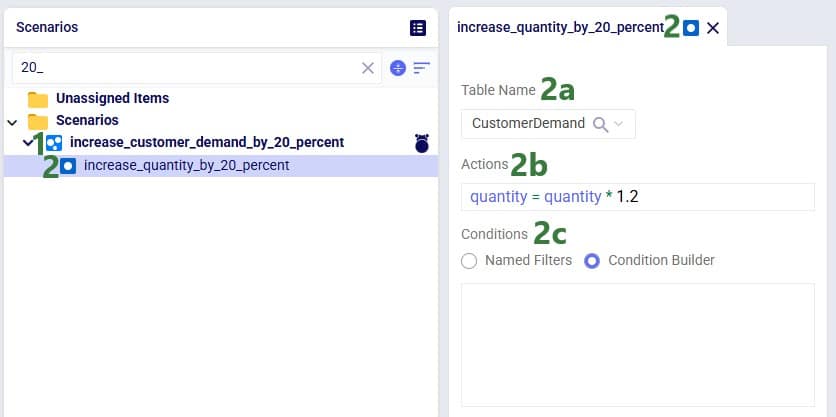
Note that if desired, the scenario and scenario item names auto-generated by Leapfrog can be changed in the Scenarios module of Cosmic Frog: just select the scenario or item and then choose “Rename” from the Scenario drop-down list at the top.
As a final example of a question & answer pair in this section, let us look at one where we use the Anura Help LLM, and Leapfrog responds with text plus context:
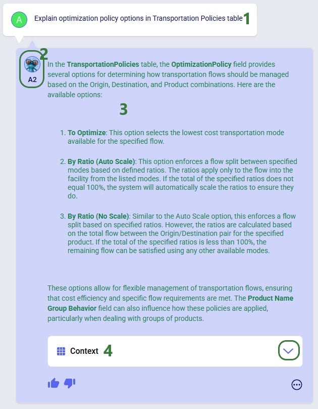
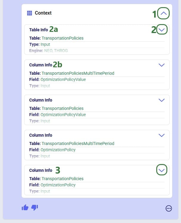
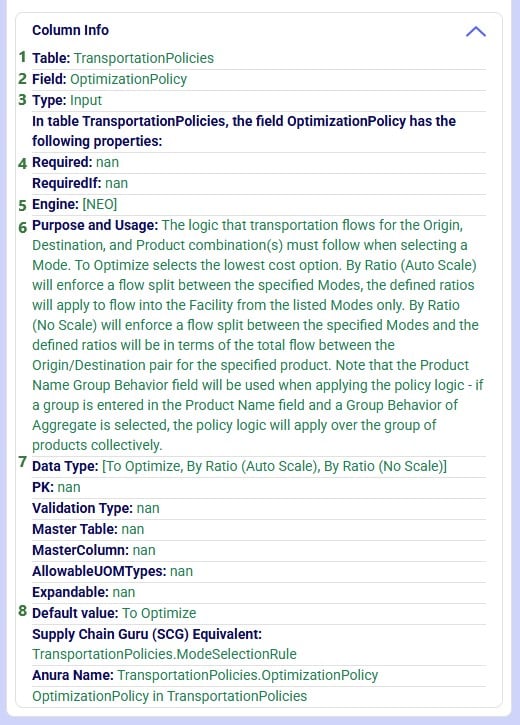
There is a lot of information listed here; we will explain the most commonly used information:
Prompts and their responses are organized into conversations in the Leapfrog module:
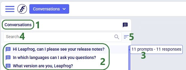
Users can organize their conversations with Leapfrog by using the options from the Conversations drop-down at the top of the Leapfrog module:
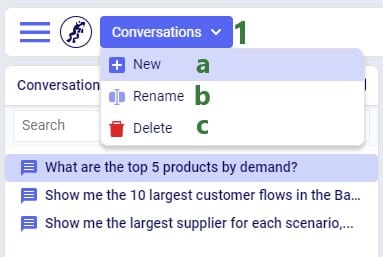
Users can rate Leapfrog responses by clicking on the thumbs up (like) and thumbs down (dislike) buttons and, optionally, providing additional feedback. This feedback is used to continuously improve Leapfrog. Giving a thumbs up to indicate the response is what you expected helps reinforce correct answers from Leapfrog. When a response is not what was expected or wrong, users can help improve Leapfrog’s underlying LLMs by giving the response a thumbs down. Especially thumbs down ratings & additional feedback will be reviewed so Leapfrog can learn and become more useful all the time.
When a response is not as expected as was the case in the following screenshot, user is encouraged to click the thumbs down button:

After clicking on the Send button, the detailed feedback is automatically added to the conversation:

The next screenshot shows an example where user gave Leapfrog’s response a thumbs up as it was what user expected. This feedback can then be used by Leapfrog to reinforce correct answers. User also had the option to provide detailed feedback again, using any of the following 4 optional tags: Showcase Example, Surprising, Fun, and Repeatable Use Case. In this example, user decided not to give detailed feedback and clicked on the Close button after the detailed feedback form came up:
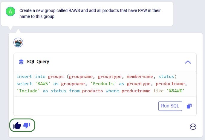
If you have any additional Leapfrog feedback (or questions) beyond what can be captured here, you can feel free to send an email to Leapfrog@Optilogic.com. You are also very welcome to ask questions, share your experiences, and provide feedback on Leapfrog in the Frogger Pond Community.
We will now go back to our first prompt “What are the top 3 products by demand” to explore some of the options users have when Data Grids are included in a Leapfrog response, which is the case when Leapfrog’s SQL Query response is a SELECT statement.
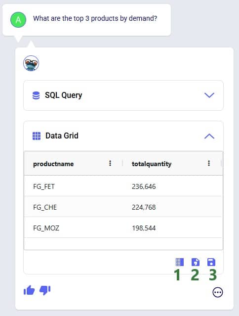


When clicking on the Download File button, a zip file with the name of the active Cosmic Frog model appended with an ID, is downloaded to the user’s Downloads folder. The zip contains:
After clicking on Save, following message appears beneath the Data Grid in Leapfrog’s response:

Looking in the Custom Tables section (#2 in screenshot below) of the Data module (#1 in screenshot below), we indeed see this newly created table named top3products (#3 in screenshot below) with the same contents as the Data Grid of the Leapfrog response:

If we choose to save the Data Grid as a view instead of a table, it goes as follows:
We choose Save as View and give it the name of Top3Products_View. The message that comes up once the view is created reads as follows:

Going to the Analytics module in Cosmic Frog, choosing to add a new dashboard and in this new dashboard a new visualization, we can find the top3products_view in the Views section:

We will go back to the original Data Grid in Leapfrog’s response to explore a few more options user has here:
Please note:
In this section we will list out what Leapfrog is capable of and give examples of each capability. These capabilities include (the LLM each capability applies to is listed in parentheses):
Each of these capabilities will be discussed in the following sections, where a brief description of each capability is given, several example prompts illustrating the capability are listed, and a few screenshots showing the capability are included as well. Please remember that many more example prompts can be found in the Prompt Library on the Frogger Pond community.
Interrogate input and output data using natural language. Use it to check completeness of input data, and to summarize input and/or output data. Leapfrog responds with SELECT Statements and shows a Data Grid preview as we have seen above. Export the data grid or save it as a table or view for further use, which has been covered above already too.
Example prompts:
The following 3 screenshots show examples of checking input data (first screenshot), and interrogating output data (second and third screenshot):
Tell Leapfrog what you want to edit in the input data of your Cosmic Frog model, and it will respond with UPDATE, INSERT, and DELETE SQL Statements. User can opt to run these SQL Queries to permanently make the change in the master input data. For UPDATE SQL Queries, Leapfrog’s response will also include the option to create a scenario and scenario item that will make the change, which we will focus on in the next section.
Example prompts:
The following 3 screenshots show examples changing values in the input data (first screenshot), adding records to an input table (second screenshot), and deleting records from an input table (third screenshot):
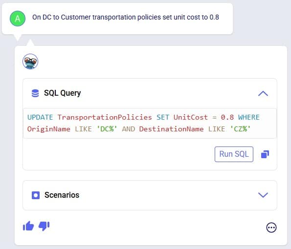
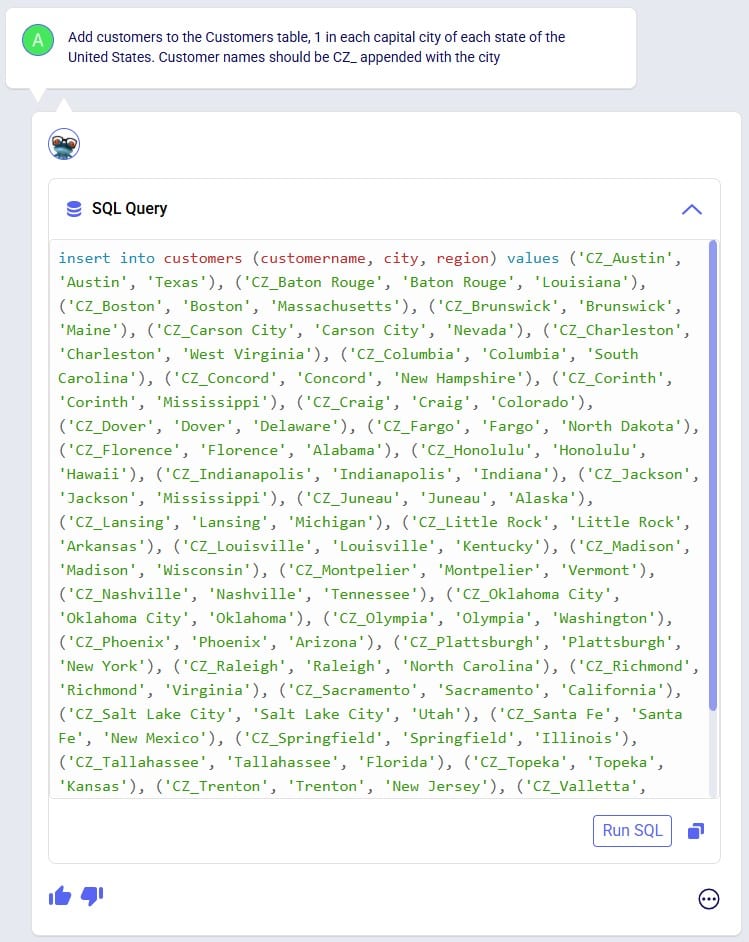
Make changes to input data, but through scenarios rather than updating the master tables directly. Prompts that result in UPDATE SQL Queries will have a Scenarios part in their responses and users can easily create a new scenario that will make the input data change by one click of a button.
Example prompts:
The following 3 screenshots show example prompts with responses from which scenarios can be created: create a scenario which makes a change to all records in 1 input table (first screenshot), create a scenario which makes a change to records in 1 input table that match a condition (second screenshot), and create a scenario that makes changes in 2 input tables (third screenshot):
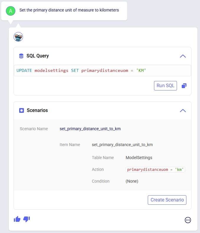
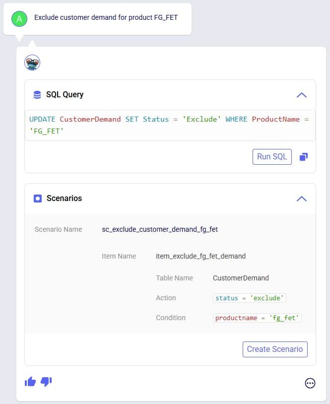
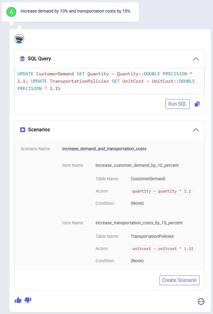
The above screenshots show examples of Leapfrog responses that contain a Scenarios section and from which new scenarios and scenario items can be created by clicking on the Create Scenario button. In addition to the above, users can also use Leapfrog to manage scenarios by using prompts that specifically create scenarios and/or items and assigning specific scenario items to specific scenarios. These result in INSERT INTO SQL Statements which can then be implemented by using the Run SQL button. See the following 2 screenshots for examples of this, where 1) a new scenario is created and an existing scenario item is then assigned to it, and 2) a new scenario item is created which is then assigned to an already existing scenario:
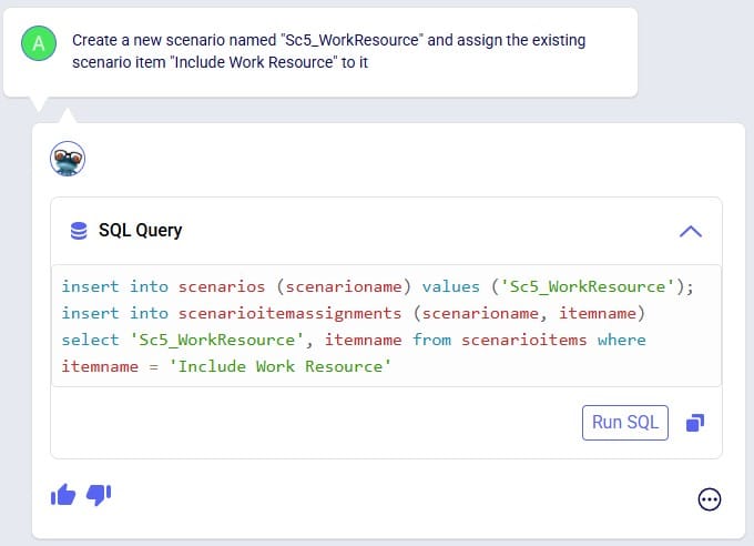
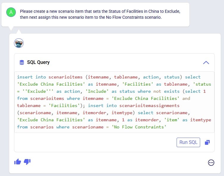
Leapfrog can create new groups and add group members to new and existing groups. Just specify the group name and which members it needs to have in the prompt and Leapfrog’s response will be one or multiple INSERT INTO SQL Statements.
Example prompts:
The following 4 screenshots show example prompts of creating groups and group members: 1) creates a new products group and adds products that have names with a certain prefix (FG_) to it, 2) creates a new periods group and adds 3 specific periods to it, 3) creates a new suppliers group and adds all suppliers that are located in China to it, and 4) adds a new member to an existing facilities group, and in addition explicitly sets the Status and Notes field of this new record in the Groups table:
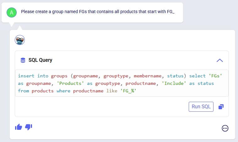
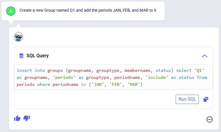

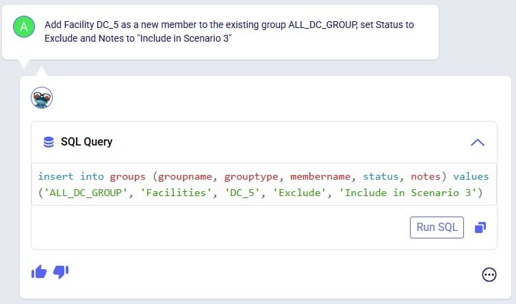
Leapfrog can create a new, blank model. Leapfrog's response will ask user to confirm if they want to create the new model before creating it. If confirmed, the response will update to contain a link which takes user to the Leapfrog module in this newly created model in a new tab of the browser.
Example prompts:
Following 2 screenshots show an example where a new model named “FrogsLeaping” is created:
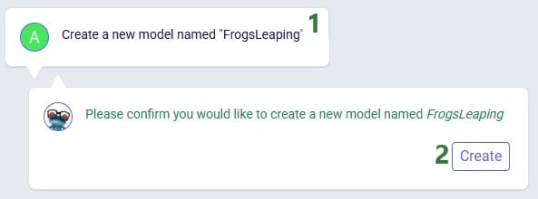
You can ask Leapfrog to kick off any model runs for you. Optionally you can specify the scenario(s) you want to be run, which engine to use, and what resource size to use. For Neo (network optimization) runs, user can additionally indicate if the infeasibility check should be turned on. If no scenario(s) are specified, all scenarios present in the model will be run. If no engine is specified, the Neo engine (network optimization) will be used. If no resource size is specified, S will be used. If for Neo runs it is not specified if the infeasibility check should be turned on or off it will be off by default.
Leapfrog’s response will summarize the scenario(s) that are to be run, the engine that will be used, the resource size that will be used, and for Neo runs if the infeasibility check will be on or off. If user indeed wants to run the scenario(s) with these settings, they can confirm by clicking on the Run button. If so, the response will change to contain a link to the Run Manager application on Optilogic’s platform, which will be opened in a new tab of the browser when clicked. In the Run Manager, users can monitor the progress of any model runs.
The engines available in Cosmic Frog are:
The resource sizes available are as follows, from smallest to largest: Mini, 4XS, 3XS, 2XS, XS, S, M, L, XL, 2XL, 3XL, 4XL, Overkill. Guidance on choosing a resource size can be found here.
Example prompts:
The following 2 screenshots show an example prompt where the response is to run the model: only the scenario name is specified in which case a network optimization (Neo) is run using resource size S with the infeasibility check turned off (False):
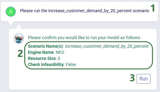
Leapfrog's response now indicates the run has been kicked off and provides a link (click on the word "here") to check the progress of the scenario run(s) in the Run Manager.
The next screenshot shows a prompt asking to specifically run Greenfield (Triad) on 2 scenarios, where the resource size to be used is specified in the prompt too:
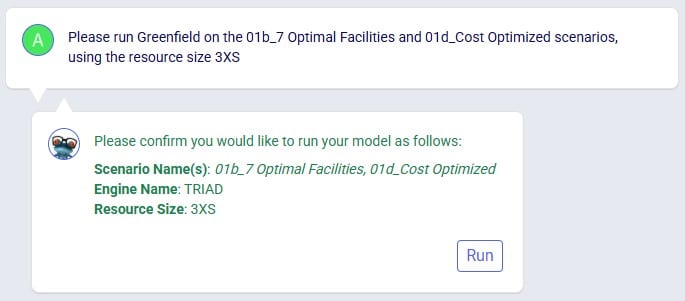
The last screenshot in this section shows a prompt to run a specific scenario with the infeasibility check turned on:
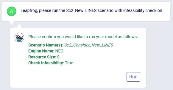
Leapfrog can find latitude & longitude pairs for locations (customers, facilities, and suppliers) based on the location information specified in these input tables (e.g. Address, City, Region, Country). Leapfrog’s response will ask user to confirm they want to geocode the specified table(s). If so, the response will change to contain a link which will open a Cosmic Frog map showing the locations that have been geocoded in a new tab of the browser.
Example prompts:
Notes on using Leapfrog for geocoding locations:
In the following screenshot, user asks Leapfrog to geocode customers:
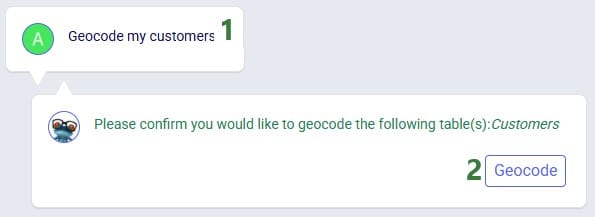
As geocoding a larger set of locations can take some time, it may look like the geocoding was not done or done incompletely if looking at the map or in the Customers / Facilities / Suppliers input tables shortly after kicking off the geocoding. A helpful tool which shows the progress of the geocoding (and other tools / utilities within Cosmic Frog) is the Model Activity list:
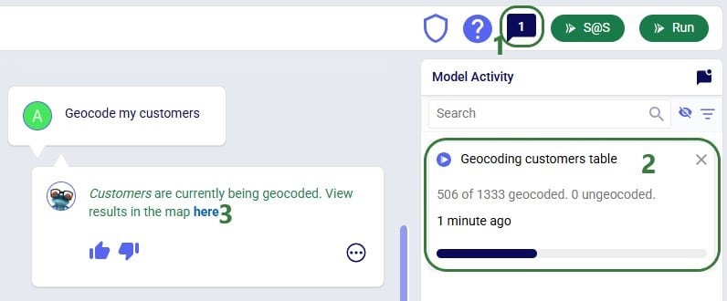
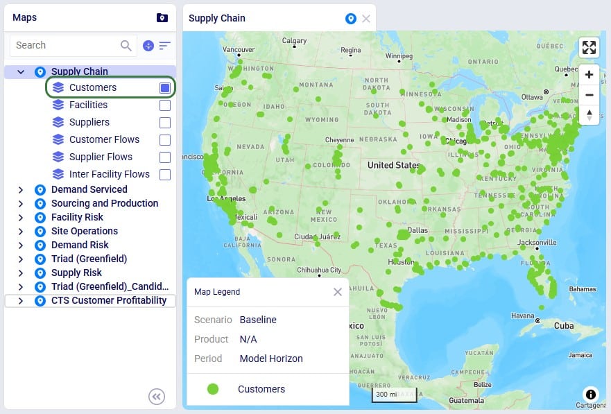
Leapfrog can teach users all about the Anura schema that underlies Cosmic Frog models, including:
Example prompts:
The following 4 screenshots show examples of these types of prompts & Leapfrog’s responses: 1) ask Leapfrog to teach us about a specific field on a specific table, 2) find out which table to use for a specific modelling construct, 3) understand the SCG to Cosmic Frog’s Anura mapping for a specific field on a specific table, and 4) ask about breaking changes in the latest Anura schema update:
Anura Help provides information around system integration, which includes:
Example prompts:
The following 4 screenshots show examples of these types of prompts & Leapfrog’s responses: 1) ask which tables are required to run a specific engine, 2) find out which engines use a specific table, 3) learn which table contains a certain type of outputs, and 4) ask about availability of template models for a specific purpose:
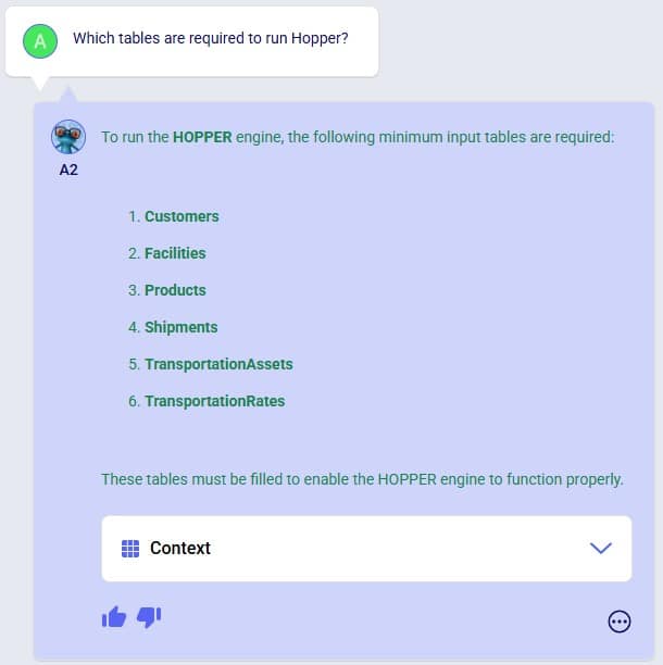


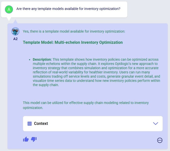
Leapfrog knows about itself, Optilogic, Cosmic Frog, the Anura database schema, LLM’s, and more. Ask Leapfrog questions so it can share its knowledge with you. For most general questions both LLMs will generate the same or a very similar answer, whereas for questions that are around capabilities, each may only answer what is relevant to it.
Example prompts:
The following 5 screenshots show examples of these types of prompts & Leapfrog’s responses: 1) ask both LLMs about their version, 2) ask a general question about how to do something in Cosmic Frog (Text2SQL), 3) ask Anura Help for the Release Notes, and 4 & 5) ask both LLMs about what they are good at and what they are not good at:

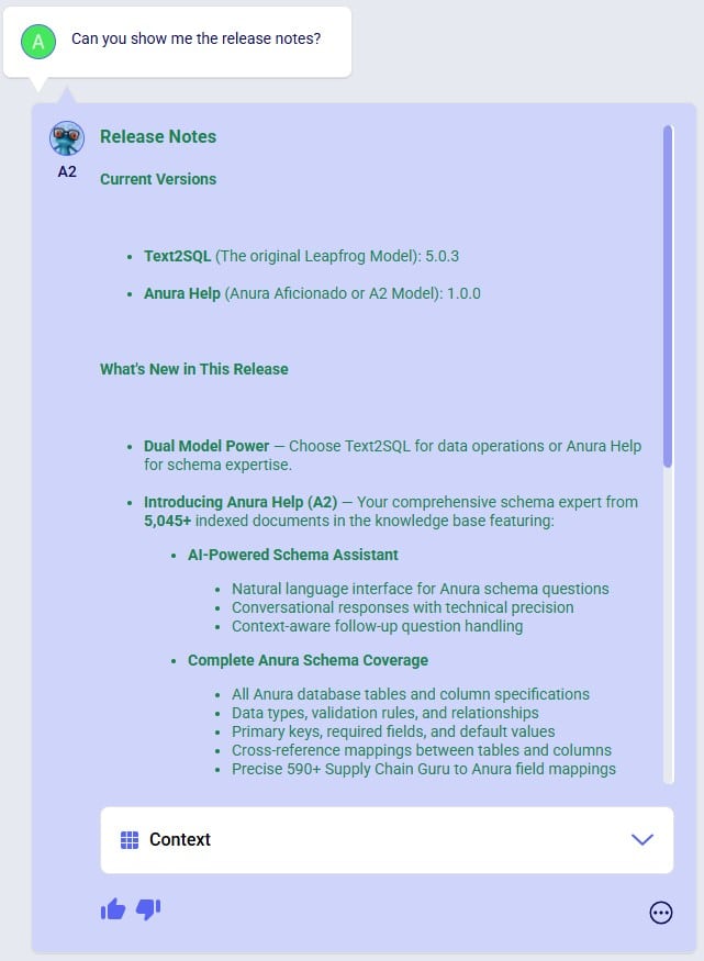
Even though this documentation and Leapfrog example prompts are predominantly in English, Leapfrog supports many languages so users can ask questions in their most natural language. Where the Leapfrog response is in text form, it can respond in the language the question was asked in. Other response types like a standard message with a link or names of scenarios and scenario items will be in English.
The following 3 screenshots show: 1) a list of languages Leapfrog supports, 2) a French prompt to increase demand by 20%, and 3) a Spanish prompt asking Leapfrog to explain the Primary Quantity UOM field on the Model Settings table:

To get the most out of Leapfrog, please take note of these tips & tricks:

After this is turned on, you can start using it by pressing the keyboard’s Windows key + H. A bar with a microphone which shows messages like “initializing”, “listening”, “thinking” will show up at the top of your active monitor:

Now you can speak into your computer’s microphone, and your spoken words will be turned into text. If you put your cursor in Leapfrog’s question / prompt area, click on the microphone in the bar at the top so your computer starts listening, and then say what you want to ask Leapfrog, it will appear in the prompt area. You can then click on the send icon to submit your prompt / question to Leapfrog.
The following screenshots show several examples of how one can build on previous prompts and responses and try to re-direct Leapfrog as described in bullets 6 and 7 of the Tips & Tricks above. In the first example user wants to delete records from an input table whereas Leapfrog’s initial response is to change the Status of these records to Exclude. The follow-up prompt clarifies that user wants to remove them. Note that it is not needed to repeat that it is about facilities based in the USA, which Leapfrog still knows from the previous prompt:
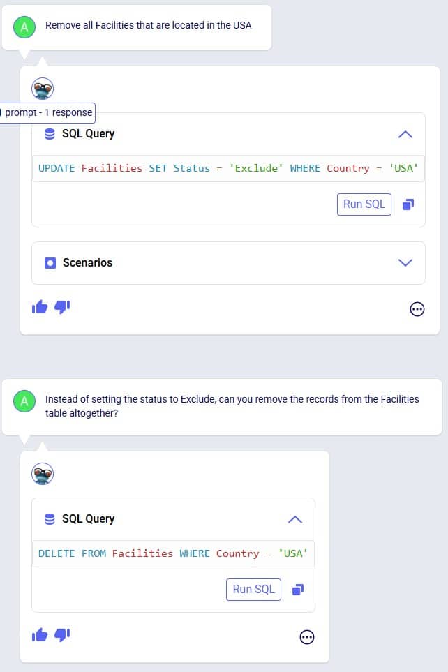
In the following example shown in the next 3 screenshots, user starts by asking Leapfrog to show the 2 DCs with the highest throughput. The SQL query response only looks at Replenishment flows, but user wants to include Customer Fulfillment flows too. Also, the SQL Query does not limit the list to the top 2 DCs. In the follow-up prompt the user clarifies this (“Like that, but…”) without needing to repeat the whole question. However, Leapfrog only picks up on the first request (adding the Customer Fulfillment flows), so in the third prompt user clarifies further (again: “Like that, but…”), and achieves what they set out to do:
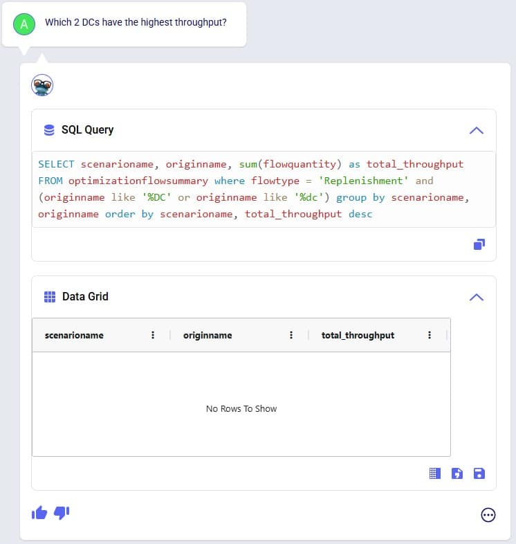
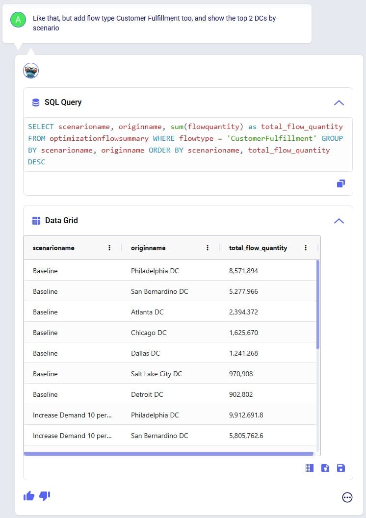
In the next 2 screenshots we see an example of first asking Leapfrog to show outputs that meet certain criteria (within 3%), and then essentially wanting to ask the same question but with the criteria changed (within 6%). There is no need to repeat the first prompt, it suffices to say something like “How about with [changed criteria]?”:
When Leapfrog only does part of what a user intends to do, it can often still be achieved in multiple steps. See the following screenshots where user intended to change 2 fields on the Production Count Constraints table and initially Leapfrog only changes one. The follow-up prompt simply consists of “And [change 2]”, building on the previous prompt. In the third prompt user was more explicit in describing the 2 changes and then Leapfrog’s response is what user intended to achieve:

Here we will step through the process of building a complete Cosmic Frog demo model, creating an additional scenario, running this new scenario and the Baseline scenario, and interrogating some of the scenarios’ outputs, all by using only Leapfrog.
Please note that if you are trying the same steps using Leapfrog in your Cosmic Frog:
We will first list the prompts that were used to build, run, and analyze the model, and then review the whole process step-by-step through (lots of!) screenshots. Here is the list of prompts that were submitted to Leapfrog (all of them used the Text2SQL LLM):
And here is the step-by-step process shown through screenshots, starting with the first prompt given to Leapfrog to create a new empty Cosmic Frog model with the name “US Distribution”:

Clicking on the link in Leapfrog’s response will take user to the Leapfrog module in this newly created US Distribution model:
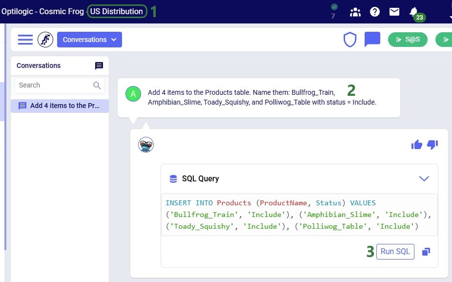
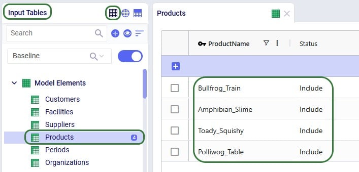
In the next prompt (the third one from the list), distribution center (DC) and manufacturing (MFG) locations are added to the Facilities table, and customer locations to the Customers table. Note the use of a numbered list to help Leapfrog break the response up into multiple INSERT INTO statements:
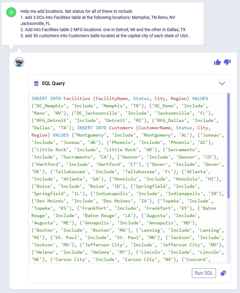
After running the SQL of that Leapfrog response, user has a look in the Facilities and Customers tables and notices that as expected all Latitude and Longitude values are blank:
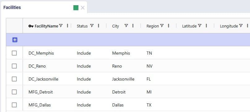
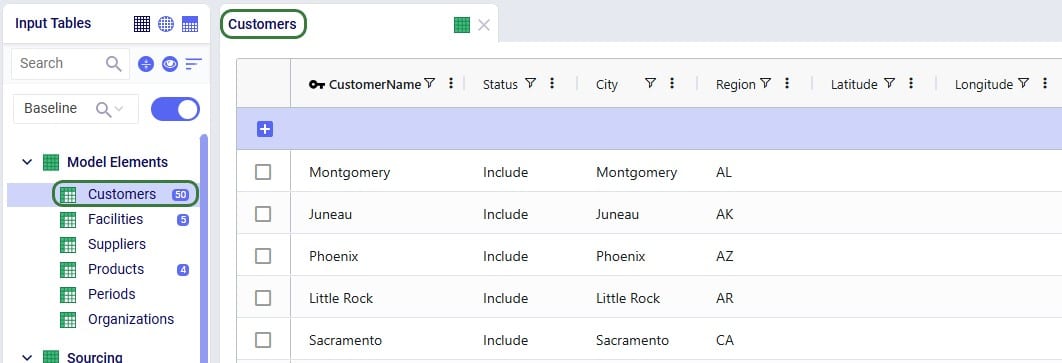
Since all Facilities and Customers have blank Latitudes and Longitudes, our next (fourth) prompt is to geocode all sites:
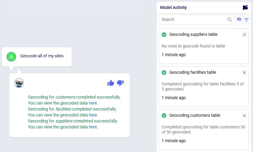
Once the geocoding completes (which can be checked in the Model Activity list), user clicks on one of the links in the Leapfrog response. This opens the Supply Chain map of the model in a new tab in the browser, showing Facilities and Customers, which all look to be geocoded correctly:
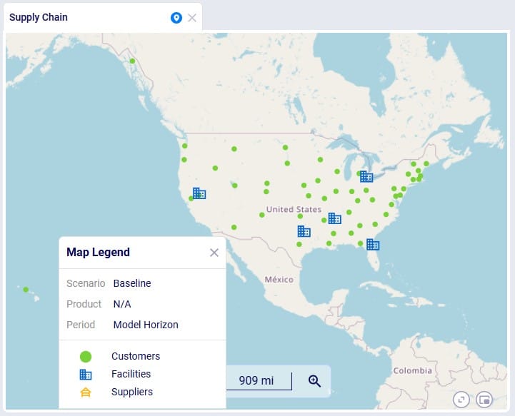
We can also double-check this in the Customers and Facilities tables, see for example next screenshot of a subset of 5 customers which now have values in their Latitude and Longitude fields:
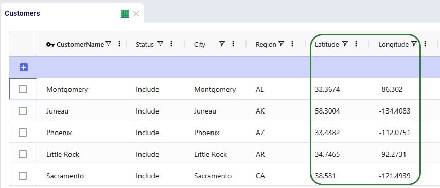
For a (network optimization - Neo) model to work, we will also need to add demand. As this is an example/demo model, we can use Leapfrog to generate random demand quantities for us, see this next (fifth) prompt and response:
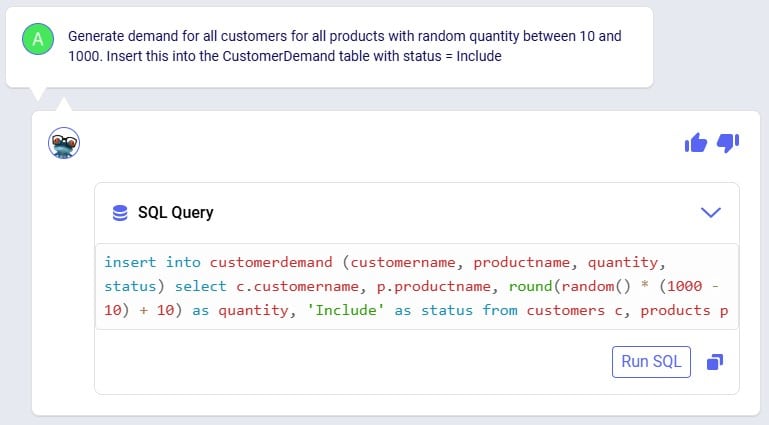
After clicking the Run SQL button, we can have a look in the Customer Demand input table, where we find the expected 200 records (50 customers which each have demand for 4 products) and eyeballing the values in the Quantity field we see the numbers are as expected between 10 and 1000:
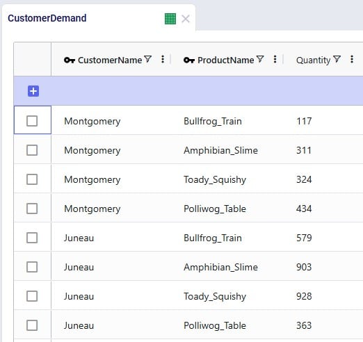
Our sixth prompt sets the model end and start dates, so the model horizon is all of 2025:
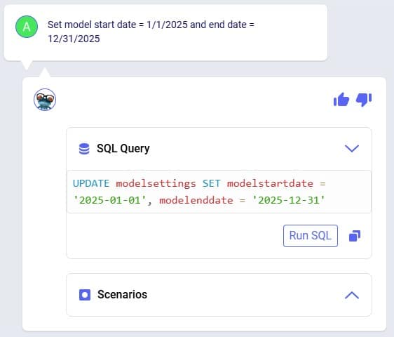
Again, we can double-check this after running the SQL response by having a look in the Model Settings input table:
We also need Transportation Policies, the following prompt (the seventh from our list) takes care of this and creates lanes from all MFGs to all DCs and from all DCs to all customers:

We see the 6 enumerated MFG (2 locations) to DC (3 locations) lanes when opening and sorting the Transportation policies table, plus the first few records of the 150 enumerated DC to customer lanes. No Unit Costs are set so far (blank values):
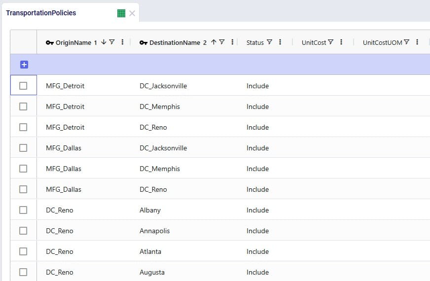
Our eighth prompt sets the transportation unit costs on the transportation policies created in the previous step. All use a unit of measure of EA-MI which means the costs entered are per unit per mile, and the cost itself is 1 cent on MFG to DC lanes and 2 cents on DC to customer lanes:
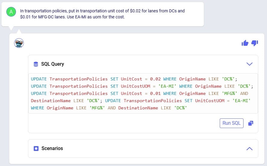
Clicking the Run SQL button will run the 4 UPDATE statements, and we can see the changes in the Transportation Policies input table:
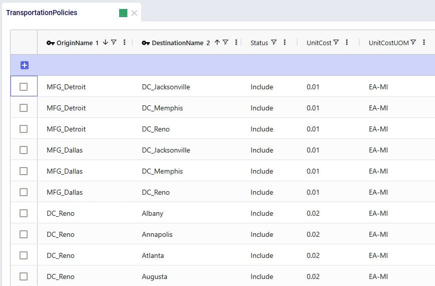
In order to run, the model also needs Production Policies, which the next (ninth) prompt takes care of: both MFG locations can produce all 4 products:
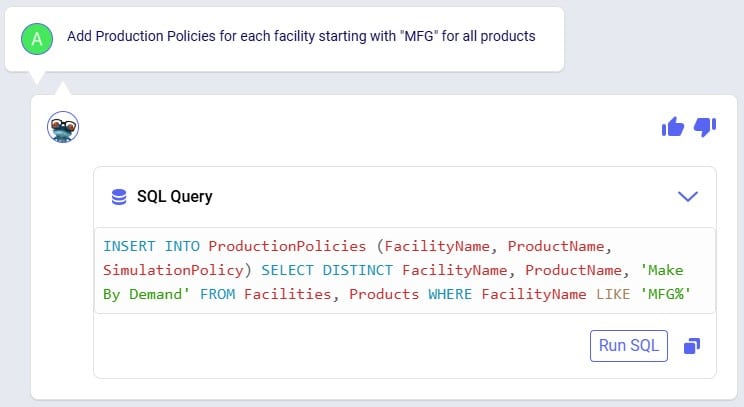
Again, double-checking after running the SQL from the response, we see the 8 expected records in the Production Policies input table:
Our 3 DCs have an upper limit as to how much throughput they can handle over the year, this is 50,000 for the DCs in Reno and Memphis and 100,000 for the DC in Jacksonville. Prompt number 10 sets these:
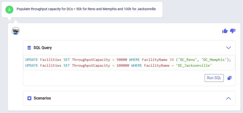
We can see these numbers appear in the Throughput Capacity field on the Facilities input table after running the SQL of Leapfrog’s response:

We want to explore what happens if the maximum throughput of the DC in Memphis is increased to 100,000; this is what the eleventh prompt asks to do:
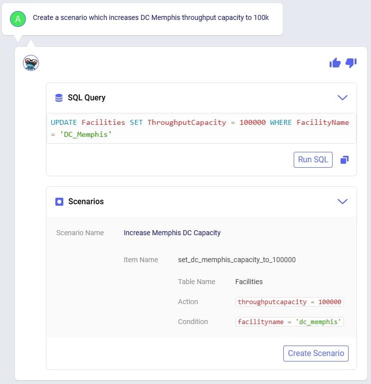
Leapfrog’s response has both a SQL UPDATE query, which would change the throughput at DC_Memphis in the Facilities input table, and a Scenarios section. We choose to click on the Create Scenario button so a new scenario is created (Increase Memphis DC Capacity) which will contain 1 scenario item (set_dc_memphis_capacity_to_100000) that sets the throughput capacity at DC_Memphis to 100,000:
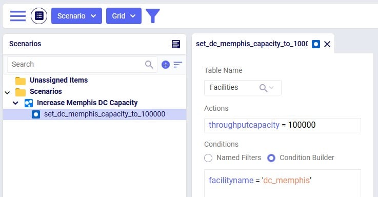
Our small demo model is now complete, and we will use Leapfrog (using our twelfth prompt) to run network optimization (using the Neo engine) on the Baseline and Increase Memphis DC Capacity scenarios:
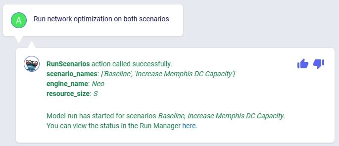
While the scenarios are running, we are thinking about what will be interesting outputs to review, and ask Leapfrog about how one can compare customers flows between scenarios (prompt number 13):
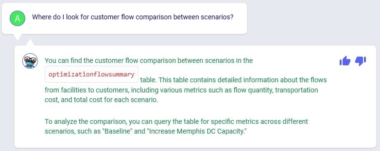
This information can come in handy in one of the next prompts to direct Leapfrog on where to look.
Using the link from the previous Leapfrog response where we started the optimization runs for both scenarios, we open the Run Manager in a new tab of the browser. Both scenarios have completed successfully as their State is set to Done:

Looking in the Optimization Network Summary output table, we also see there are results for both scenarios:
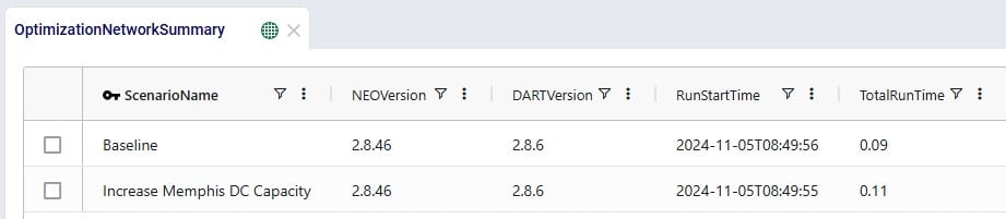
In the next few prompts Leapfrog is used to look at outputs of the 2 scenarios that have been run. The prompt (number 14 from our list) in the next screenshot aims to get Leapfrog to show us which customers have a different source in the Increase Memphis DC Capacity scenario as compared to the Baseline scenario:
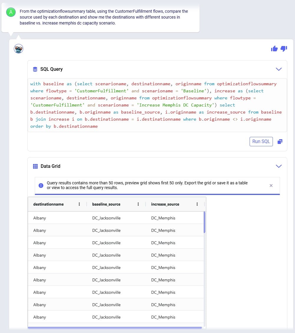
Leapfrog’s response is almost what we want it to be, however it has duplicates in the Data Grid. Therefore, we follow our previous prompt up with the next one (number 15), where we ask to see only distinct combinations. Instead of “distinct” we could have also used the word “unique” in our prompt:
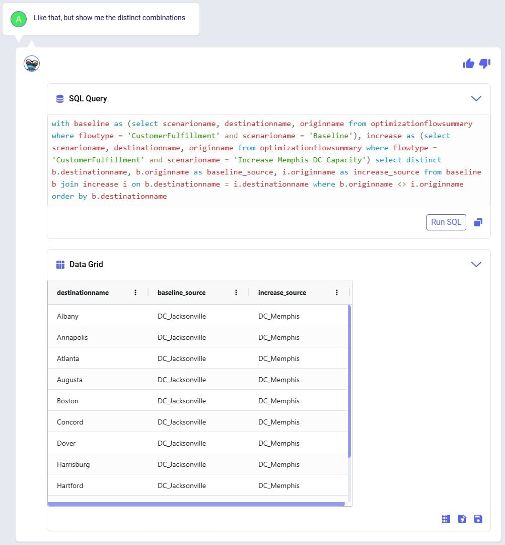
We see that the source for around 11-12 customers changed from the DC in Jacksonville in the Baseline to the DC in Memphis in the Increase Memphis DC Capacity scenario.
Cost comparisons between scenarios are usually interesting too, so that is what prompt number 16 asks about:
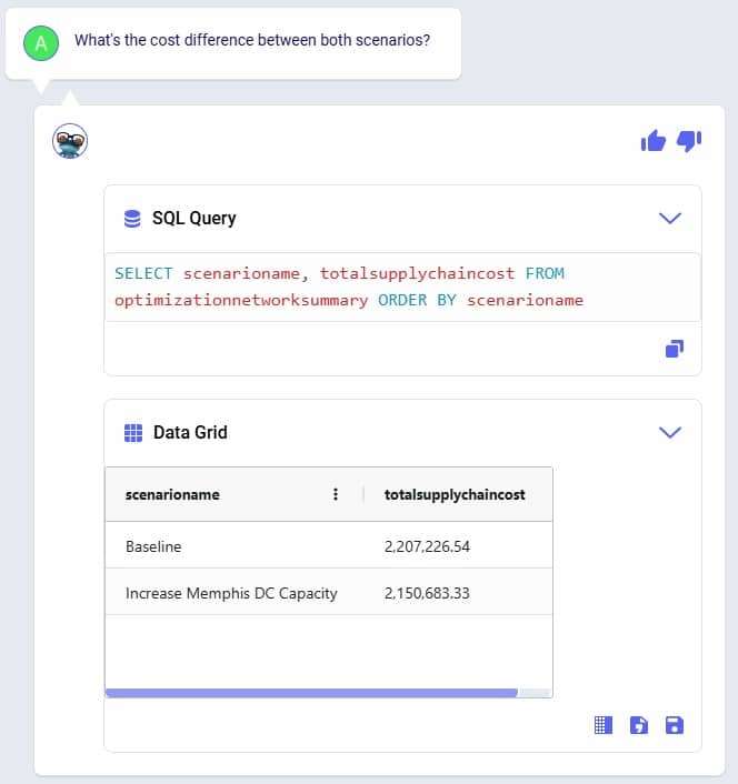
We notice that increasing the throughput capacity at DC_Memphis leads to a lower total supply chain cost by about 56.5k USD. Next, we want to see how much flow has shifted between the DCs in the Baseline scenario compared to the Increase Memphis DC Capacity scenario, which is what the last prompt (number 17) asks about:
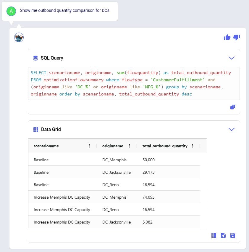
This tells us that the throughput at DC_Reno is the same in both scenarios, but that increasing the DC_Memphis throughput capacity allows a shift of about 24k units from the DC in Jacksonville to the DC in Memphis (which was at its maximum 50k throughput in the Baseline scenario). This volume shift is what leads to the reduction in total supply chain cost.
We hope this gives you a good idea of what Leapfrog is capable of today. Stay tuned for more exciting features to be added in future releases!
Do you have any Leapfrog questions or feedback? Feel free to use the Frogger Pond Community to ask questions, share your experiences, and provide feedback. Or, shoot us an email at Leapfrog@Optilogic.com.
Happy Leapfrogging!
PERSONA: Alex is an experienced supply chain modeler who knows exactly what to analyze but often spends too much time pulling and formatting outputs. They are looking to be more efficient in summarizing results and identifying key drivers across scenarios. While confident in their domain expertise, they want help extracting insights faster without losing control or accuracy. They see AI as a time-saving partner that helps them focus on decision-making, not data wrangling.
USE CASE: After running multiple scenarios in Cosmic Frog, Alex wants to quickly understand the key differences in cost and service across designs. Instead of manually exporting data or writing SQL queries, Alex uses Leapfrog to ask natural-language questions which saves Alex hours and lets them focus on insight generation and strategic decision-making.
Model to use: Global Supply Chain Strategy (available under Get Started Here in the Explorer).
Prompt #1
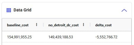
Prompt #2
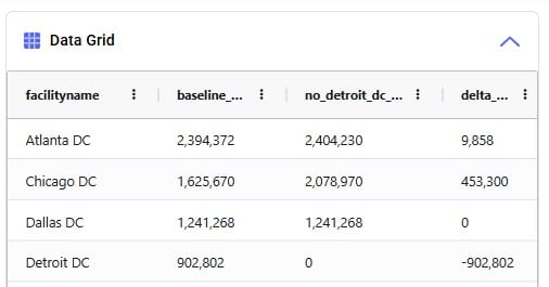
Prompt #3
Prompt #4
Prompt #5
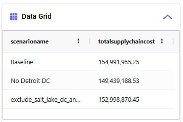
PERSONA: Chris is an experienced supply chain modeler with a well-established, repeatable workflow that pulls data from internal systems to rebuild models every quarter. He relies on consistency in the model schema to keep his automation running smoothly.
USE CASE: With an upcoming schema change in Cosmic Frog, Chris is concerned about disruptions or errors in his process and wants Leapfrog to help provide info on the changes that may require him to update his workflow.
Model to use: any.
Prompt #1
Prompt #2
Prompt #3
PERSONA: Larry Loves LLMs – he wants to use an LLM to find answers.
USE CASE: I need to understand the outputs of this model someone else built. I want to know how many products come from each supplier for each network configuration. Can Leapfrog help with that?
Yes, Leapfrog can help with that! Let's use Anura Help to better understand which tables have that data and then ask Text2SQL to pull the data.
Model to use: any; Global Supply Chain Strategy (available under Get Started Here in the Explorer).
Prompt #1
Prompt #2
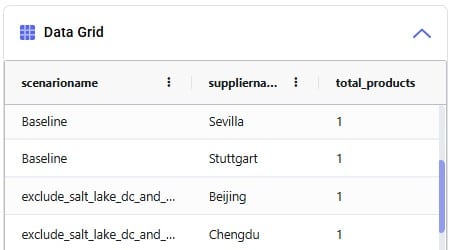
To enable users to build basic Cosmic Frog for Excel Applications to interact directly with Cosmic Frog from within Excel without needing to write any code, Optilogic has developed the Cosmic Frog for Excel Application Builder (also referred to as App Builder in this documentation). In this App Builder, users can build their own workflows using common actions like creating a new model, connecting to an existing model, importing & exporting data, creating & running scenarios, and reviewing outputs. Once a workflow has been established, the App can be deployed so it can be shared with other users. These other users do not need to build the workflow of the App again, they can just use the App as is. In this documentation we will take a user through the steps of a complete workflow build, including App deployment.
You can download the Cosmic Frog for Excel – App Builder from the Resource Library. A video showing how the App Builder is used in a nutshell is included; this video is recommended viewing before reading further. After downloading the .zip file from the Resource Library and unzipping it on your local computer, you will find there are 2 folders included: 1) Cosmic_Frog_For_Excel_App_Builder, which contains the App Builder itself and this is what this documentation will focus on, and 2) Cosmic_Frog_For_Excel_Examples, which contains 3 examples of how the App Builder can be used. This documentation will not discuss these examples in detail; users are however encouraged to browse through them to get an idea of the types of workflows one can build with the App Builder.
The Cosmic_Frog_For_Excel_App_Builder folder contains 1 subfolder and 1 Macro-enabled Excel file (.xlsm):

When ready to start building your first own basic App, open the Cosmic_Frog_For_Excel_Builder_v1.xlsm file; the next section will describe the steps a user needs to take to start building.
When you open the Cosmic_Frog_For_Excel_App_Builder_v1.xlsm file in Excel, you will find there are 2 worksheets present in the workbook, Start and Workflow. The top of the Start worksheet looks like this:
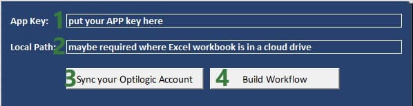
Going to the Workflow worksheet and clicking on the Cosmic Frog tab in the ribbon, we can see the actions that are available to us to create our basic Cosmic Frog for Excel Applications:

We will now walk through building and deploying a simple App to illustrate the different Actions and their configurations. This workflow will: connect to a Greenfield model in my Optilogic account, add records to the Customer and CustomerDemand tables, create a new scenario with 2 new scenario items in it, run this new scenario, and then export the Greenfield Facility Summary output table from the Cosmic Frog model into a worksheet of the App. As a last step we will also deploy the App.
On the Workflow worksheet, we will start building the workflow by first connecting to an existing model in my Optilogic account:

The following screenshot shows the Help tab of the “Connect To Or Create Model Action”:
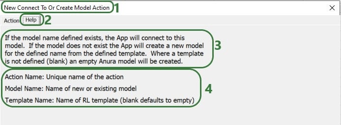
In the remainder of the documentation, we will not show the Help tab of each action. Users are however encouraged to use these to understand what the action does and how to configure it.
After creating an action, the details of it will be added to 2 columns in the Workflow worksheet, see screenshot below. The first action of the workflow will use columns A & B, the next action C & D, etc. When adding actions, the placement on the Workflow worksheet is automatic and user does not need to do or change anything. Blue fields contain data that cannot be changed, white fields are user inputs when setting up the action and can be changed in the worksheet itself too.

The United States Greenfield Facility Selection model we are connecting to contains about 1.3k customer locations in the US which have demand for 3 products: Rockets, Space Suits, and Consumables. As part of this workflow, we will add 10 customers located in the state of Ontario in Canada to the Customers table and add demand for each of these customers for each product to the CustomerDemand table. The next 2 screenshots show the customer and customer demand data that will be added to this existing model.
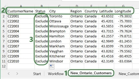

First, we will use an Import Data action to append the new customers to the Customers table in the model we are connecting to:
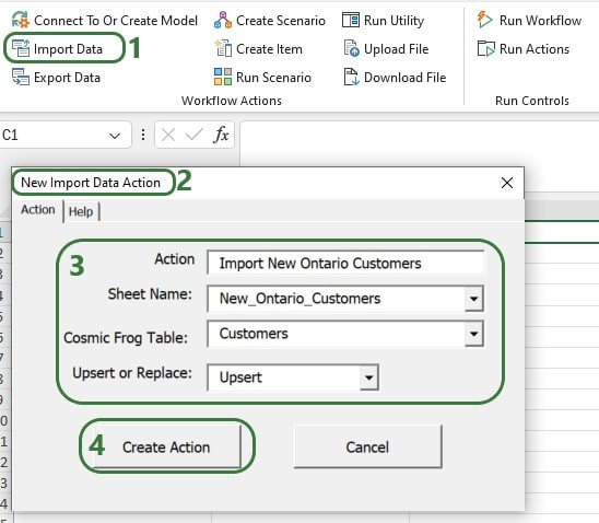
Next, use the Import Data Action again to upsert the data contained in the New_CustomerDemand worksheet to the CustomerDemand table in the Cosmic Frog model, which will be added to columns E & F. After these 2 Import Data actions have been added, our workflow now looks like this:

Now that the new customers and their demand have been imported into the model, we will add several actions to create a new scenario where the new customers will be included. In this scenario, we will also remove the Max Number of New Facilities value, so the Greenfield algorithm can optimize the number of new facilities just based on the costs specified in the model. After setting up the scenario, an action will be added to run it.
Use the Create Scenario action to add a new scenario to the model:
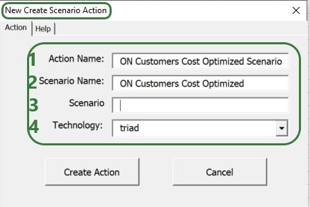
Then, use 2 Create Item Actions to 1) include the Ontario customers and 2) remove the Max Number Of New Facilities value:
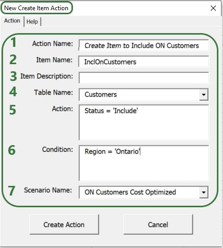
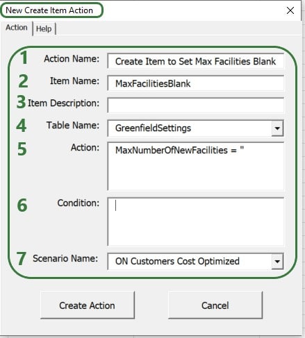
After setting up the scenario and its 2 items, the next step of the workflow will be to run it. We add a Run Scenario action to the workflow to do so:
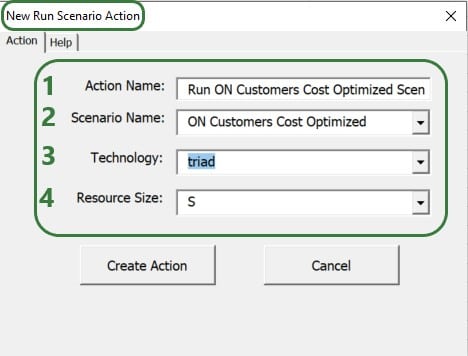
The configuration of this action takes following inputs:
We now have a workflow that connects to an existing US Greenfield model, adds Ontario customers and their demand to this model, then creates and runs a new scenario with 2 items in this Cosmic Frog model. After running the scenario, we want to export the Optimization Greenfield Facility Summary output table from the Cosmic Frog model and load it into a new worksheet in the App. We do so by adding an Export Data Action to the workflow:
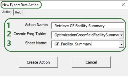
After adding the above actions to the workflow, the workflow worksheet now looks like the following 2 screenshots from column G onwards (columns A-F contain the first 3 actions as shown in a screenshot further above):

Columns G-H contain the details of the action that created the new ON Customers Cost Optimized scenario, and columns I-J & K-L contain the details of the actions that added the 2 scenario items to this scenario.

Columns M-N contain the details of the action that will run the scenario that was added and columns O-P those of the action that will export the selected output table (Optimization Greenfield Facility Summary) into the GF_Facility_Summary worksheet of the App.
To run the completed Workflow, all we need to do is click on the Run Workflow action and confirm we want to run it:
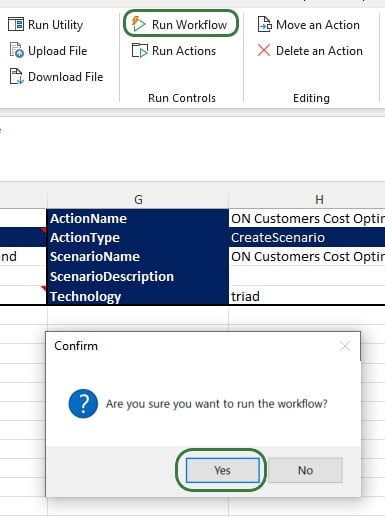
After kicking off the workflow, if we switch to the Start worksheet, details of the run and its progress are shown in rows 9-11:

Looking on the Optilogic Platform, we can also check the progress of the App run and the Cosmic Frog model changes:
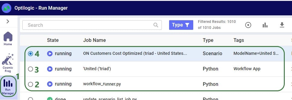
Once the run is done all 3 jobs will have their State changed to Done, unless an error occurred in which case the State will say Error.
Checking the United Stated Greenfield Facility Selection model itself in the Cosmic Frog application on cosmicfrog.com:
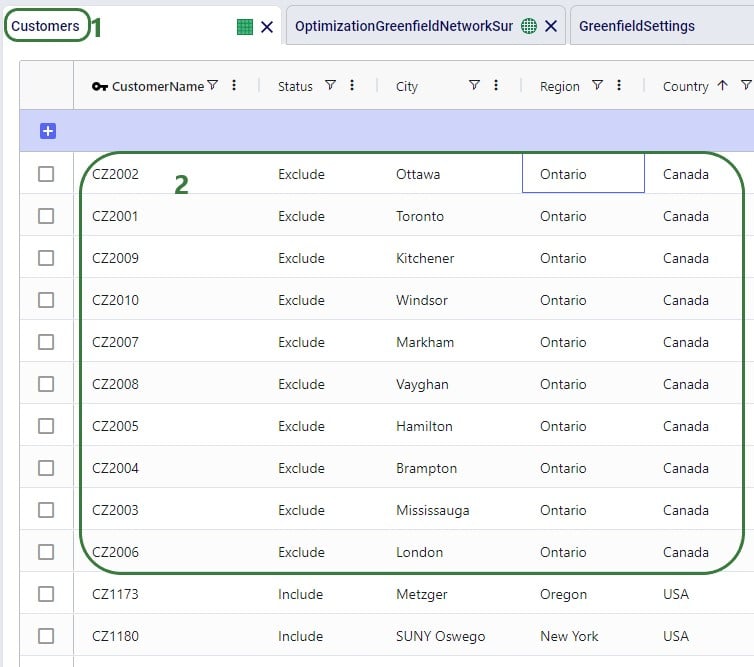
Once the App is finished running, we see that a worksheet named GF_Facility_Summary was added to the App Builder:
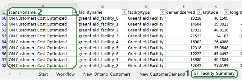
There are several other actions that users of the App Builder can incorporate into a workflow or use to facilitate workflow building. We will cover these now. Feel free to skip ahead to the “Deploying the App” section if your workflow is complete at this stage.
Additional actions that can be incorporated into workflows are the Run Utility, Upload File, and Download File actions. The Run Utility action can be used to run a Cosmic Frog Utility (a Python script), which currently can be a Utility downloaded from the Resource Library or a Utility specifically built for the App.
There are currently 4 Utilities available in the Resource Library:

After downloading the Python file of the Utility you want to use in your workflow, you need to copy it into the working_files_do_not_change folder that is located in the same folder as where you saved the App Builder. Now you can start using it as part of the Run Utility action. In the below example, we will use the Python script from the Copy Map to a Model Resource Library Utility to copy a map and all its settings from one model (“United States Greenfield Facility Selection”, the model connected to in a previous action) to another (“European Greenfield Facility Selection”):
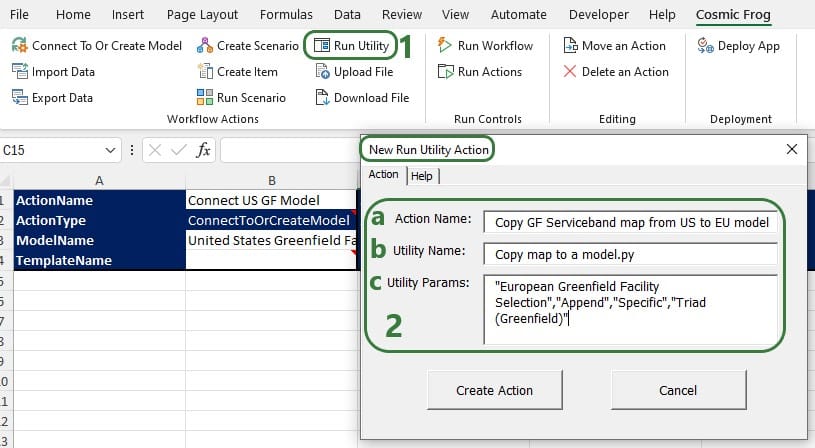
The parameters of the Copy Dashboard to a Model Utility are the same as those of the Copy Map to a Model Utility:
The Orders to Demand and Delete SaS Scenarios utilities do not have any parameters that need to be set, so the Utility Params part of the Run Utility action can be left blank when using these utilities.
The Upload File action can be used to take a worksheet in the App Builder and upload it as a .csv file to the Optilogic platform:
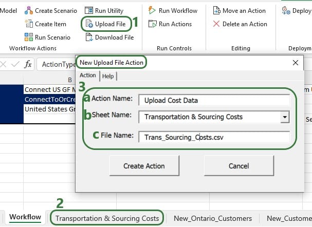
Files that get uploaded to the Optilogic platform are placed in a specific working folder related to the App Builder, the name and location of which are shown in this screenshot:

The Download File action can be used to download a .txt file from the Optilogic platform and load it into a worksheet in the App:
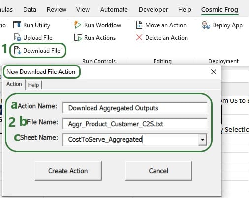
Other actions that facilitate workflow building are the Move an Action, Delete an Action, and Run Actions actions, which will be discussed now. If the order of some actions needs to be changed, you do not need to remove and re-add them, you can use the Move an Action action to move them around:

It is also possible that an action needs to be removed from a Workflow. For this, the “Delete an Action” action can be used, rather than manually deleting it from the Workflow worksheet and trying to move other actions in its place:
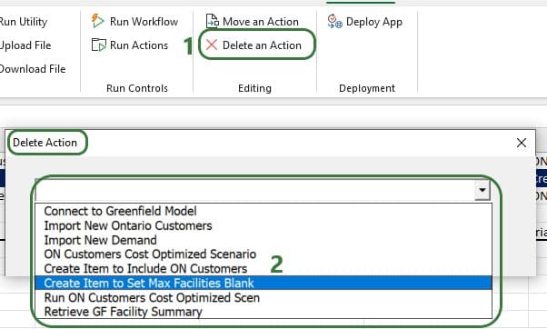
Instead of running a complete workflow, it is also possible to only run a subset of the actions that are part of the workflow:

Once a workflow has been completed in the Cosmic Frog for Excel App Builder, it can be deployed so other users can run the same workflow without having to build it first. This section covers the Deployment steps.
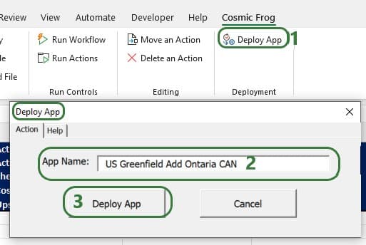
The following message will come up after the app had been deployed:
Looking in the folder mentioned in this message, we see the following contents:
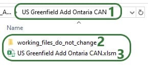

Congratulations on building & deploying your own Cosmic Frog for Excel App!
If you want to build Apps that go beyond what can be done using the App Builder, you can do so too. This may require some coding using Excel VBA, Python, and/or SQL. Detailed documentation walking through this can be found in this Getting Started with Cosmic Frog for Excel Applications article on Optilogic’s Help Center.
Teams is an exciting new feature set designed to enhance collaboration within Supply Chain Design, enabling companies to foster a more connected and efficient working environment. With Teams, users can join a shared workspace where all team members have seamless access to collective models and files. This ensures that every piece of work remains synchronized, providing a single source of truth for your data. When one team member updates a file, those changes instantly reflect for all other members, eliminating inconsistencies and ensuring that everyone stays aligned.
Beyond simply improving collaboration, Teams offers a structured and flexible way to organize your projects. Instead of keeping all your files and models confined to a personal account, you can now create distinct teams tailored to different projects, departments, or business functions. This means greater clarity and easier navigation between workspaces, ensuring that the right content is always at your fingertips.
Consider the possibilities:
Teams introduces a more intuitive and structured way to collaborate, organize, and access your work—ensuring that your team members always have the latest updates and a streamlined experience. Get started today and transform the way you work together!
This documentation contains a high-level overview of the Teams feature set, details the steps to get started, gives examples of how Teams can be structured, and covers best practices. More detailed documentation for Organization Administrators and Teams Users is available in the following help center articles:
The diagram below highlights the main building blocks of the Teams feature set:
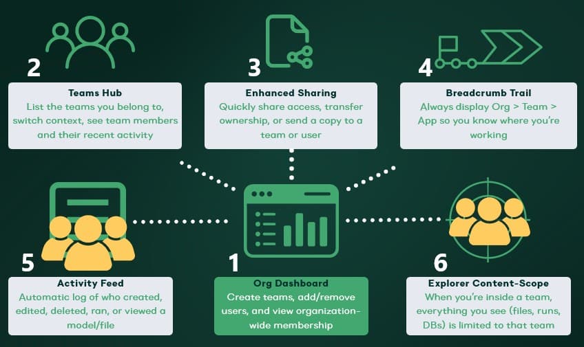
At a high-level, these are the steps to start using the Teams feature set:
Here follow 5 examples of how teams can be structured, including an example for each and an explanation of why such a setup works well.
Please keep following best practices in mind to ensure optimal use of the Teams feature set:
Once you have set up your teams and added content, you are ready to start collaborating and unlocking the full potential of Teams within Optilogic!
Let us know if you need help along the way—our support team (support@optilogic.com) has your back.
Depending on the type of supply chain one is modelling in Cosmic Frog and the questions being asked of it, it may be necessary to utilize some or all the features that enable detailed production modelling. A few business case examples that will often include some level of detailed production modelling include:
In comparison, modelling a retailer who buys all its products from suppliers as finished goods, does not require any production details to be added to its Cosmic Frog model. Hybrid models are also possible, think for example of a supermarket chain which manufactures its own branded products and buys other brands from its suppliers. Depending on the modelling scope, the production of the own branded products may require using some of the detailed production features.
The following diagram shows a generalized example of production related activities at a manufacturing plant, all of which can be modelled in Cosmic Frog:

In this help article we will cover the inputs & outputs of Cosmic Frog’s production modelling features, while also giving some examples of how to model certain business questions. The model in Optilogic’s Resource Library that is used mainly for the screenshots in this article is the Multi-Year Capacity Planning. There is a 20-minute video available with this model in the Resource Library, which covers the business case that is modelled and some detail of the production setup too.
To not make this document too repetitive we will cover some general Cosmic Frog functionality here that applies to all Cosmic Frog technologies and is used extensively for production modelling in Neo too.
To only show tables and fields in them that can be used by the Neo network optimization algorithm, select Optimization in the Technologies Filter from the toolbar at the top in Cosmic Frog. This will hide any tables and fields that are not used by Neo and therefore simplifies the user interface.
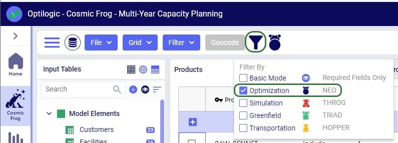
Quite a few Neo related fields in the input and output tables will be discussed in this document. Keep in mind however that a lot of this information can also be found in the tooltips that are shown when you hover over the column name in a table, see following screenshot for an example. The column name, technology/technologies that use this field, a description of how this field is used by those algorithm(s), its default value, and whether it is part of the table’s primary key are listed in the tooltip.
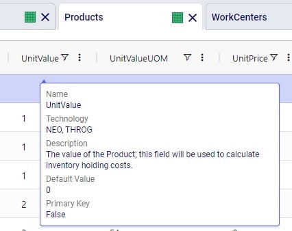
There are a lot of fields with names that end in “…UOM” throughout the input tables. How they work will be explained here so that individual UOM fields across the tables do not need to be explained further in this documentation as they all work similarly. These UOM fields are unit of measure fields and often appear to the immediate right of the field that they apply to, like for example Unit Value and Unit Value UOM in the screenshot above. In these UOM fields you can type the Symbol of a unit of measure that is of the required Type from the ones specified in the Units Of Measure input table. For example, in the screenshot above, the unit of measure Type for the Unit Value UOM field is Quantity. Looking in the Units Of Measure input table, we see there are 2 of these specified: Each and Pallet, with Symbol = EA and PLT, respectively. We can use either of these in this UOM field. If we leave a UOM field blank, then the Primary UOM for that UOM Type specified in the Model Settings input table will be used. For example, for the Unit Value UOM field in the screenshot above the tooltip says Default Value = {Primary Quantity UOM}. Looking this up in the Model Settings table shows us that this is set to EA (= each) in our current model. Let’s illustrate this with the following screenshots of 1) the tooltip for the Unit Value UOM field (located on the Products input table), 2) units of measure of Type = Quantity in the Units Of Measure input table and 3) checking what the Primary Quantity UOM is set to in the Model Settings input table, respectively:
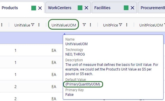

Note that only hours (Symbol = HR) is currently allowed as the Primary Time UOM in the Model Settings table. This means that if another Time UOM, like for example minutes (MIN) or days (DAY), is to be used, the individual UOM fields need to be utilized to set these. Leaving these blank would mean HR is used by default.
With few exceptions, all tables in Cosmic Frog contain both a Status field and a Notes field. These are often used extensively to add elements to a model that are not currently part of the supply chain (commonly referred to as the “Baseline”), but are to be included in scenarios in case they will definitely become part of the future supply chain or to see whether there are benefits to optionally include these going forward. In these cases, the Status in the input table is set to Exclude and the Notes field often contains a description along the lines of ‘New Market’, ‘New Line 2026’, ‘Alternative Recipe Scenario 3, ‘Faster Bottling Plant5 China’, ‘Include S6’, etc. When creating scenario items for setting up scenarios, the table can then be filtered for Notes = ‘New Market’ while setting Status = ‘Include’ for those filtered records. We will not call out these Status and Notes fields in each individual input table in the remainder of this document, but we do encourage users to use these extensively as they make creating scenarios very easy. When exploring any Cosmic Frog models in the Resource Library, you will notice the extensive use of these fields too. The following 2 screenshots illustrate the use of the Status and Notes fields for scenario creation: 1) shows several customers on the Customers table where CZ_Secondary_1 and CZ_Secondary_2 are not currently customers that are being served but we want to explore what it takes to serve them in future. Their Status is set to Exclude and the Notes field contains ‘New Market’; 2) a scenario item called ‘Include New Market’ shows that the Status of Customers where Notes = ‘New Market’ is changed to ‘Include’.
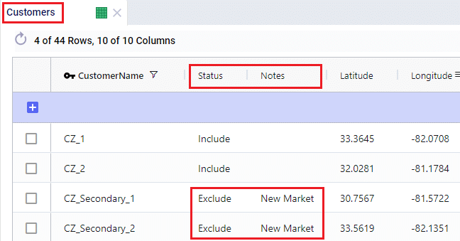
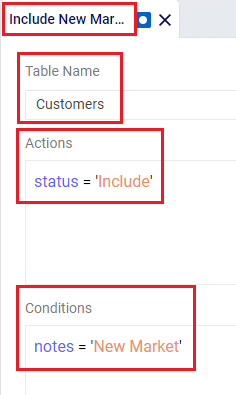
The Status and Notes fields are also often used for the opposite where existing elements of the current supply chain are excluded in scenarios in cases where for example manufacturing locations, products or lines are going to go offline in the future. To learn more about scenario creation, please see this short Scenarios Overview video, this Scenario Creation and Maps and Analytics training session video, this Creating Scenarios in Cosmic Frog help article, and this Writing Scenario Syntax help article.
The model that is mostly used for screenshots throughout this help article is as mentioned above the Multi-Year Capacity Planning model that can be found here in the Resource Library. This model represents a European cheese supply chain which is used to make investment decisions around the growth of a non-mature market in Eastern Europe over a 5-year modelling horizon. New candidate DCs are considered to serve the growing demand in Eastern Europe, the model optimizes which are optimal to open and during which of the 5 years of the modelling horizon. The production setup in the model uses quite a few of the detailed modelling features which will be discussed in detail in this document:
Note that in the screenshots of this model, the columns have been re-ordered sometimes, so you may see a different order in your Cosmic Frog UI when opening the same tables of this model.
The 2 screenshots below show the Products and Facilities input tables of this model in Cosmic Frog:
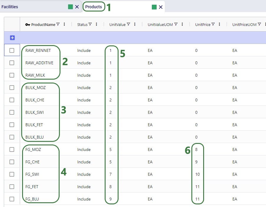
Note that the naming convention of the products lends itself to easy filtering of the table for the raw materials, bulk materials, and finished goods due to the RAW_, BULK_, and FG_ prefixes. This makes the creation of groups and setting up of scenarios quick and easy.
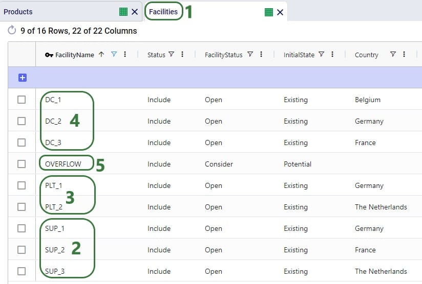
Note that similar to the naming convention of the products, the facilities are also named with prefixes that facilitate filtering of the facilities so groups and scenarios can quickly be created.
Here is a visual representation of the model with all facilities and customers on the map:

The specific features in Cosmic Frog that allow users to model and optimize production processes of varying levels of complexity while using the network optimization engine (Neo) include the following input tables:
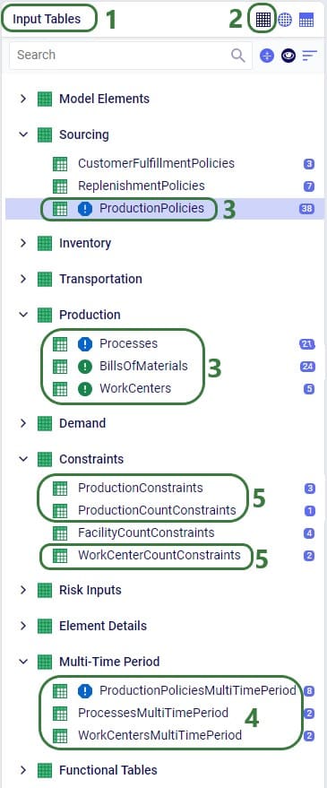
We will cover all these production related input tables to some extent in this article, starting with a short description of each of the basic single-period input tables:
These 4 tables feed into each other as follows:
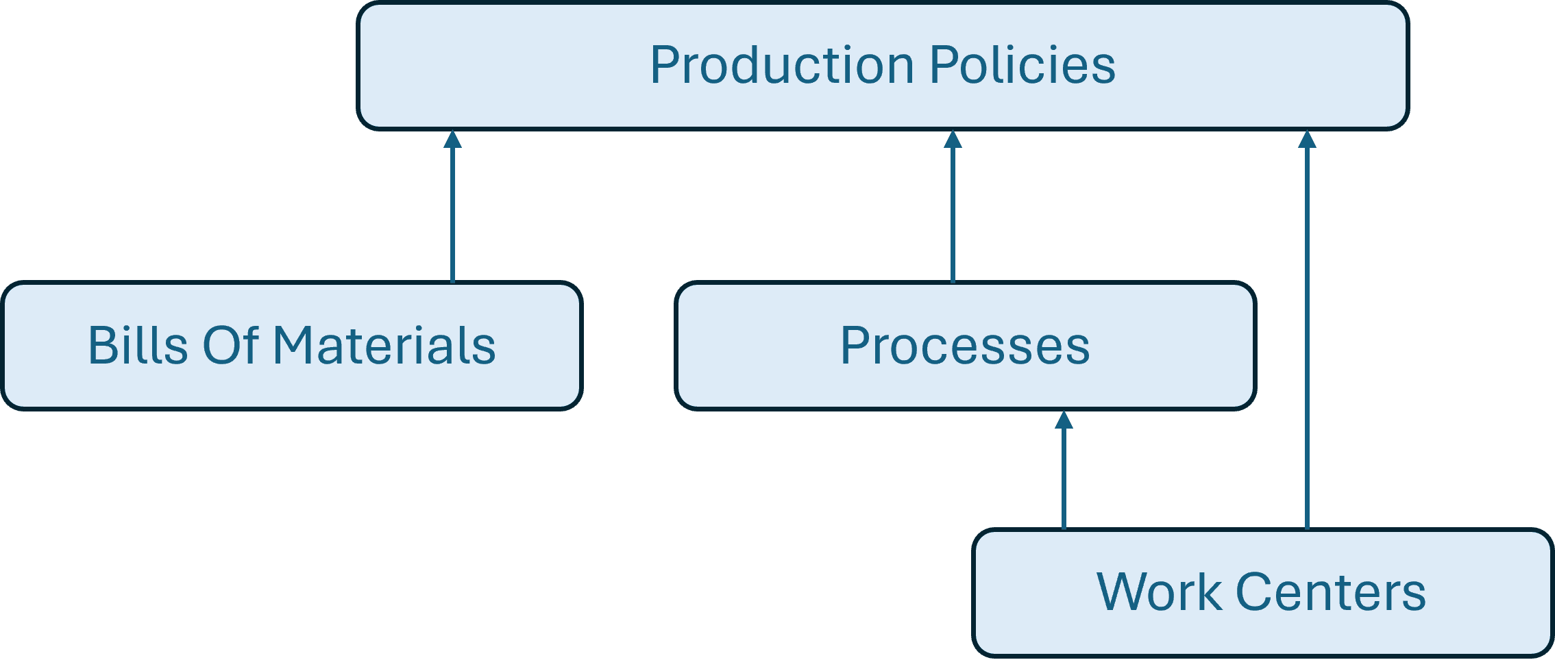
A couple of notes on how these tables work together:
For all products that are explicitly modelled in a Cosmic Frog model, there needs to be at least 1 policy specified on the Production Policies table or the Supplier Capabilities table so there is at least 1 origin location for each. This applies to for example raw materials, intermediates, bulk materials, and finished goods. The only exception is if by-products are being modelled, these can have Production Policies associated with them, but do not necessarily need to (more on this when discussing Bills of Materials further below). From the 2 screenshots below of the Production Policies table, it becomes clear that depending on the type of product and the level of detail that is needed for the production elements of the supply chain, production policies can be set up quite differently: some use only a few of the fields, while others use more/different fields.
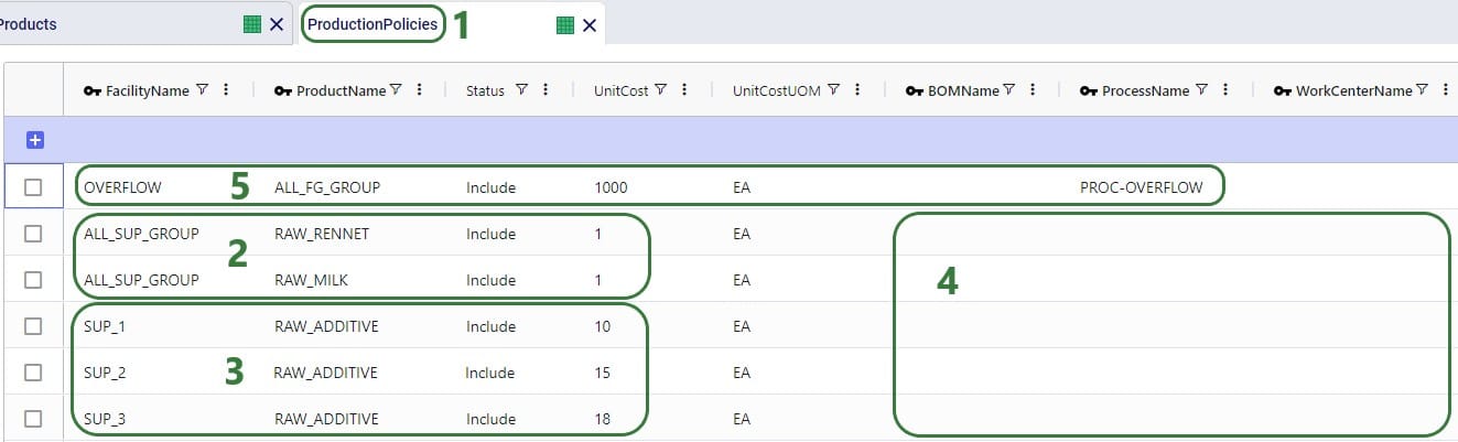
A couple of notes as follows:
Next, we will look at a few other records on the Production Policies input table:

We will take a closer look at the BOMs and Processes specified on these records when discussing the Bills of Materials and Processes tables further below.
Note that the above screenshot was just for PLT_1 and mozzarella, there are similar records in this model for the other 4 cheeses which can also be made at PLT_1, plus similar records for all 5 cheeses at PLT_2, which includes a new potential production line for future expansion too.
Other fields on the Production Policies table that are not shown in the above 2 screenshots are:
The recipes of how materials/products of different stages convert into each other are specified on the Bills of Materials (BOMs) table. Here the BOMs for the blue cheese (_BLU) products are shown:
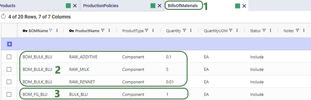
Note that the above specified BOMs are both location and end-product agnostic. Their names suggest that they are specific for making the BULK_BLU and FG_BLU products, but only associating these BOMs on a Production Policy which has Product Name set to these makes this connection. We can use these BOMs at any location that they apply. Filtering the Production Policies table for the BULK_BLU and FG_BLU products we can see that 1) BOM_BULK_BLU is indeed used to make BULK_BLU and BOM_FG_BLU to make FG_BLU, and 2) the same BOMs are used at PLT_1 and PLT_2:
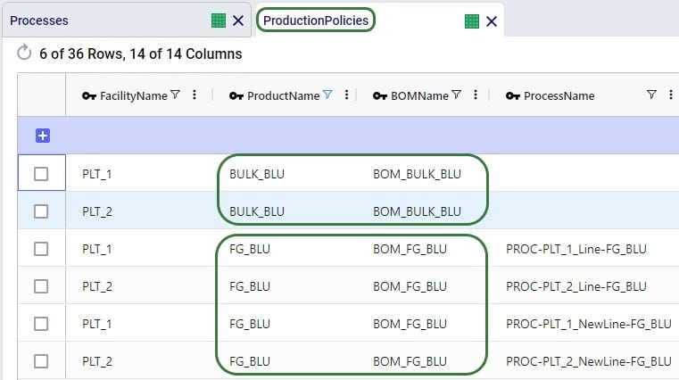
It is of course possible that the same product uses a different BOM at a different location. In this case, users can set up multiple BOMs for this product on the BOMs table and associate the correct one at the correct location in the Production Policies table. Choosing a naming convention for the BOM Names that includes the location name (or a code to indicate it) is recommended.
The screenshot above of the Bills of Materials table only shows records with Product Type = Component. Components are input into a BOM and are consumed by it when producing the end-product. Besides Component, Product Type can also be set to End Product or Byproduct. We will explain these 2 product types through the examples in this following screenshot:
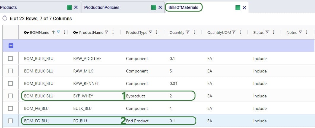
Notes:
On the Processes table production processes of varying levels of complexity can be set up, from simple 1 step processes without using any work centers, to multi-step ones that specify costs, processing rates, and use different work centers for each step. The processes specified in the Multi-Year Capacity Planning model are relatively straightforward:
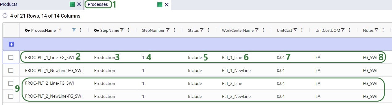
Let us also look at an example in a different model which contains somewhat more complex processes for a car manufacturer where the production process can roughly be divided into 3 steps:

Note that, like BOMs, Processes can in theory be both location and end-product agnostic. However:
Other fields on the Processes table that are not shown in the above 2 screenshots are:
If it is important to capture costs and/or capacities of equipment like production lines, tools, machines that are used in the production process, these can be modelled by using work centers to represent the equipment:
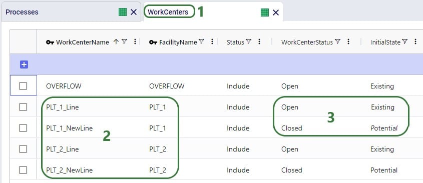
In the above screenshot, 2 work centers are set up at each plant: 1 existing work center and 1 new potential work center. The new work centers (PLT_1_NewLine and PLT_2_NewLine) have Work Center Status set to Closed, so they will not be considered for inclusion in the network when running the Baseline scenario. In some of the scenarios in the model, the Work Center Status of these 2 lines is changed to Consider and in these scenarios one of the new lines or both can be opened and used if it is optimal to do so. The scenario item that makes this change looks like this:
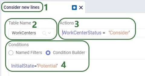
Next, we will also look at a few other fields on the Work Centers table that the Multi-Year Capacity Planning model utilizes:
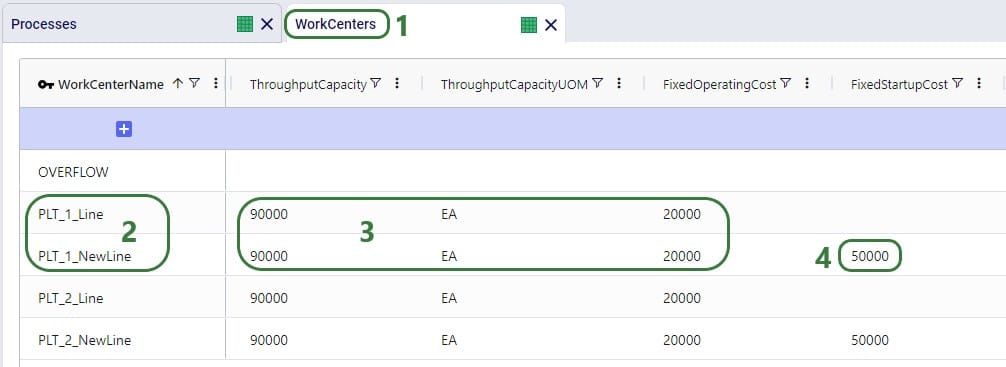
In theory, it can be optimal for a model to open a considered potential work center in one period of the model (say 2024 in this model), close it again in a later period (e.g. 2025), for it then to open it again later (e.g. 2026), etc. In this case Fixed Startup or Fixed Closing Costs would be applied each time the work center was opened or closed, respectively. This type of behavior can be undesirable and is by default prevented by a Neo Run Parameter called “Open Close At Most Once”, as shown in this screenshot:

After clicking on the Run button, the Run screen comes up. The “Open Close At Most Once” parameter can be found in the Neo (Optimization) Parameters section. By default, it is turned on, meaning that a work center or facility is only allowed to change state once during the model’s horizon, i.e. once from closed to open if the Initial State = Potential or once from open to closed if the Initial State = Existing. There may however be situations where opening and/or closing of work centers and facilities multiple times during the model horizon is allowable. In that case, the Open Close At Most Once parameter can be turned off.
Other fields on the Work Centers table that are not shown in the above screenshots are:
Fixed Operating, Fixed Startup, and Fixed Closing Costs can be stepped costs. These can be entered into the fields on the Work Centers input table directly or can be specified on the Step Costs input table and then used on the Work Centers table in those cost fields. An example of stepped costs set up in the Step Costs input table is shown in the screenshot below where the costs are set up to capture the weekly shift cost for 1 person (note that these stepped costs are not in the Multi-Year Capacity Planning model in the Resource Library, they are shown here as an additional example):
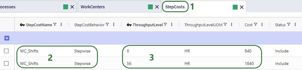
To set for example the Fixed Operating Cost to use this stepped cost, type “WC_Shifts” into the Fixed Operating Cost field on the Work Centers input table.
Many of the input tables in Cosmic Frog have a Multi-Time Period equivalent, which can be used in models that have more than 1 period. These tables enable users to make changes that only apply to specific periods of the model. For example, to:
The multi-time period tables are copies of their single-period equivalents, with a few columns added and removed (we will see examples of these in screenshots further below):
Notes on switching status of records through the multi-period tables and updating records partially:
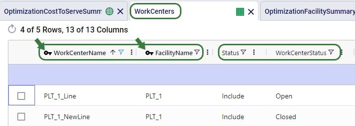
Three of the 4 production specific input tables that have been discussed above have a multi-time period equivalent: Production Policies, Processes, and Work Centers. There is no equivalent for the Bills Of Materials input table, as BOMs are only used if they are associated on records in the Production Policies table. Using different BOMs during different periods can be achieved by associating those BOMs on the Production Policies single-period table and setting the Status of them to Include for those to be used for most of the periods and to Exclude if they are to be included for certain periods / scenarios. Then add those records for which the Status needs to be switched to the Production Policies multi-period input table (we will walk through an example of this using screenshots in the next section).
The 3 production specific multi-time period input tables do have all of the same fields as their single-period equivalents, with the addition of the Period Name field and additional Status field. We will not discuss each multi-time period table and all its fields in detail here, but rather give a few examples of how each can be used.
Note that from this point onwards the Multi-Year Capacity Planning model was modified and added to for purposes of this help article, the version in the Resource Library does not contain the same data in the Multi-Time Period input tables and production specific Constraint tables that is shown in the screenshots below.
This first example on the Production Policies Multi-Time Period input table shows how the production of the cheddar finished good (FG_CHE) is prevented at plant 1 (PLT_1) in years 4 and 5 of the model:
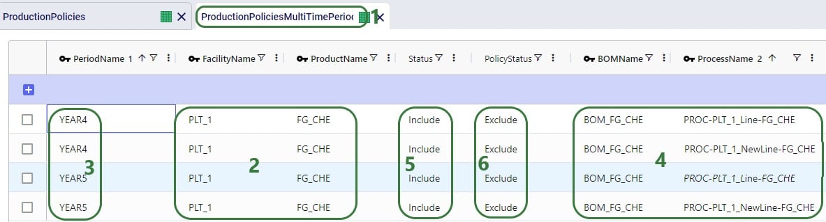
In the following example, an alternative BOM to make feta (FG_FET) is added and set to be used at Plant 2 (PLT_2) during all periods instead of the original BOM. This is set up to be used in a scenario, so the original records need to be kept intact for the Baseline and other scenarios. To set this up, we need to update the Bills Of Materials, Production Policies, and Production Policies Multi-Time Period table, see the following screenshots and explanations:

On the Bills Of Materials input table, all we need to do is add the records for the new BOM that results in FG_FET. It has 2 records, both named ALTBOM_FG_FET, and instead of using only BULK_FET as the component which is what the original BOM uses, it uses a mix of BULK_FET and BULK_BLU as its components.
Next, we first need to associate this new BOM through the Production Policies table:
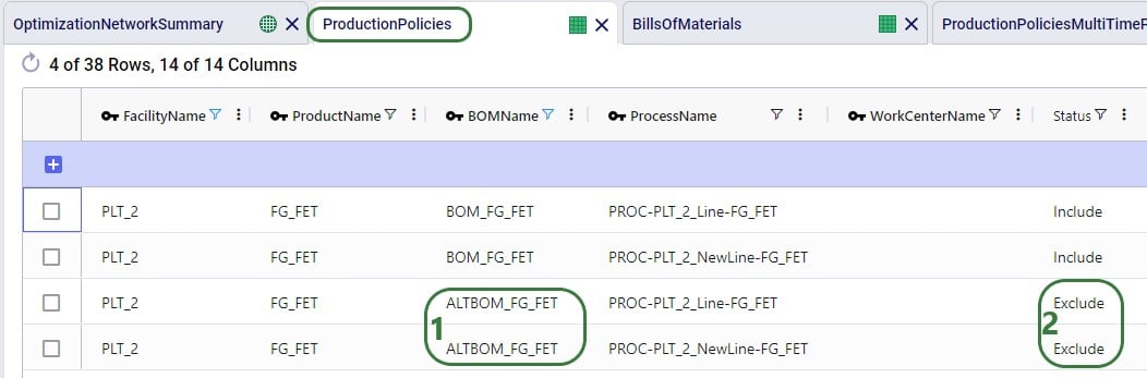
Lastly, the records that need to be added to the Production Policies Multi-Time Period table are the following 4 which have all the same values for the key columns as the 4 records in the above screenshot of the Production Policies single-period input table, which contain all the possible ways to produce FG_FET at PLT_2:
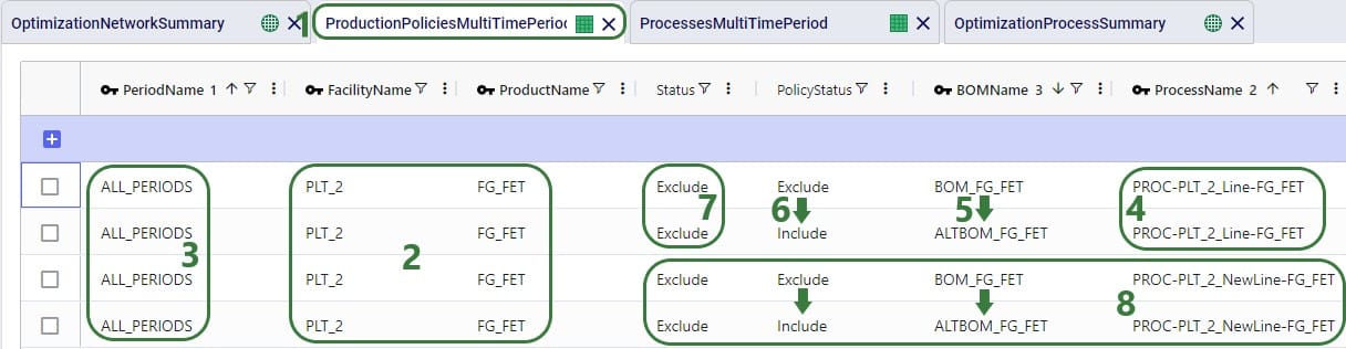
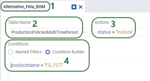
In the following example, we want to change the unit cost on 2 of the processes: at Plant 1 (PLT_1), the cost on the new potential line needs to be decreased to 0.005 for cheddar cheese (CHE) and increased to 0.015 for Swiss cheese (SWI). This can be done by using the Processes Multi-Time Period input table:
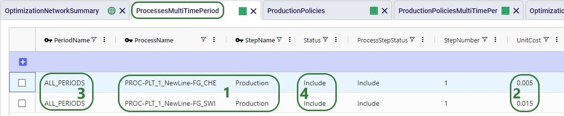
Note that there is also a Work Center Name field on the Processes Multi-Time Period table (not shown in the screenshot). As this is not a key field on the Processes input tables, it can be left blank here on the multi-time period table. This field will not be changed and the value from the single-time period table Work Center Name field will be used for these 2 records.
In the following example, we want to evaluate if upgrading the existing production lines at both plants from the 3rd year of the modelling horizon onwards, so they have a higher throughput capacity at a somewhat higher fixed operating cost, is a good alternative to opening one of the potential new lines at either plant. First, we add a new periods group to the model to set this up:
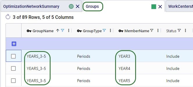
On the Groups table, we set up a new group named YEARS3-5 (Group Name) that is of Group Type = Periods and has 3 members: YEAR3, YEAR4 and YEAR5 (Member Name).

Cosmic Frog contains multiple tables through which different types of constraints can be added to network optimization (Neo) models. A constraint limits the model in a certain part of the network. These limits can for example be lower or upper limits in terms of the amount of flow between certain locations or certain echelons, the amount of inventory of a certain product or product group at a specific location or network wide, the amount of production of a certain product or product group at a specific location or network wide, etc. In this section the 3 constraints tables that are production specific will be covered: Production Constraints, Production Count Constraints, and Work Center Count Constraints.
A couple of general notes on all constraints tables:
In this example, we want to add constraints to the model that limit the production of all 5 finished goods together to 90,000 units. Both plants have this same upper production limit across the finished goods, and the limit applies to each year of the modelling horizon (5 yearly periods).

Note that there are more fields on the Production Constraints input table which are not shown in the above screenshot. These are:
In this example, we want to limit the number of products that are produced at PLT_1 to a maximum of 3 (out of the 5 finished goods). This limit applies over the whole 5-year modelling period, meaning that in total PLT_1 can produce no more than 3 finished goods:

Again, note there are more fields on the Production Count Constraints input table which are not shown in the above screenshot. These are:
Next, we will show an example of how to open at least 3 work centers, but no more than 5 out of 8 candidate work centers. These limits apply to all 5 yearly periods in the model together and over all facilities present in the model.

Again, there are more fields on the Work Center Count Constraints table that are not shown in the above screenshot:
After running a network optimization using Cosmic Frog’s Neo technology, production specific outputs can be found in several of the more general output tables, like the Optimization Network Summary, and the Optimization Constraints Summary (if any constraints were applied). Outputs more focused on just production can be found in 4 production specific output tables: the Optimization Production Summary, the Optimization Bills Of Material Summary, the Optimization Process Summary, and the Optimization Work Center Summary. We will cover these tables here, starting with the Optimization Network Summary.
The following screenshot shows the production specific outputs that are contained in the Optimization Network Summary output table:
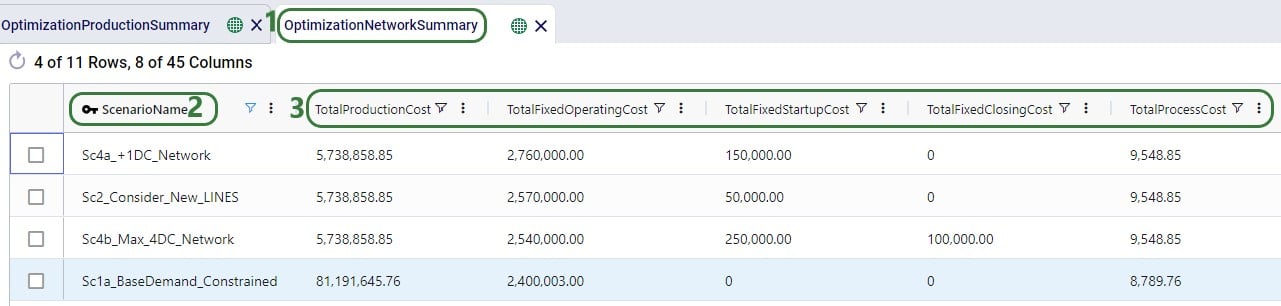
Other production related fields on this table which are not shown in the screenshot above are:
The Optimization Production Summary output table has a record with the production details for each product that was produced as part of the model run:
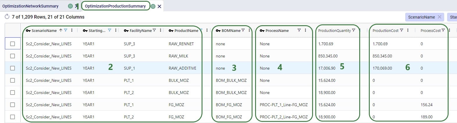
Other fields on this output table which are not shown in the screenshot are:
The details of how many components were used and how much by-product produced as a result of any bills of materials that were used as part of the production process can be found on the Optimization Bills Of Material Summary output table:
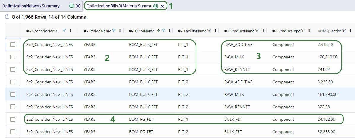
Note that aside from possibly knowing based on the BOM Name, it is not listed in the Bills Of Material Summary output table what the end product is and how much of it is produced as a result of a BOM. Those details are contained in the Optimization Production Summary output table discussed above.
Other fields on this output table which are not shown in the screenshot are:
The details of all the steps of any processes used as part of the production in the Neo network optimization run can be found in the Optimization Process Summary, see these next 2 screenshots:
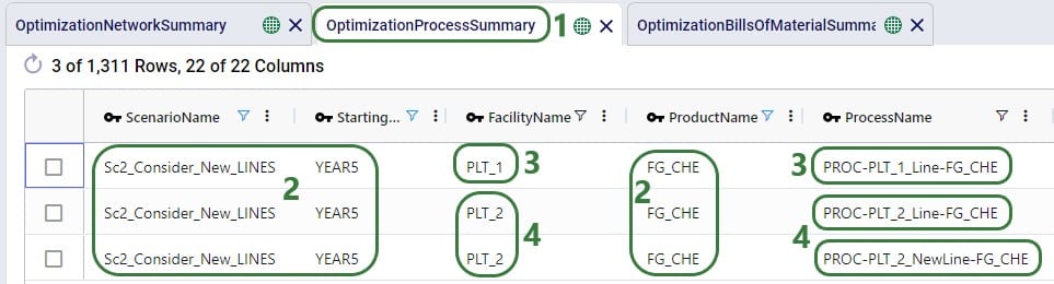

Other fields on this output table which are not shown in the screenshots are:
For each Work Center that has its Status set to Include or Consider, a record for each period of the model can be found in the Optimization Work Center Summary output table. It summarizes if the Work Center was used during that period, and, if so, how much and at what cost:
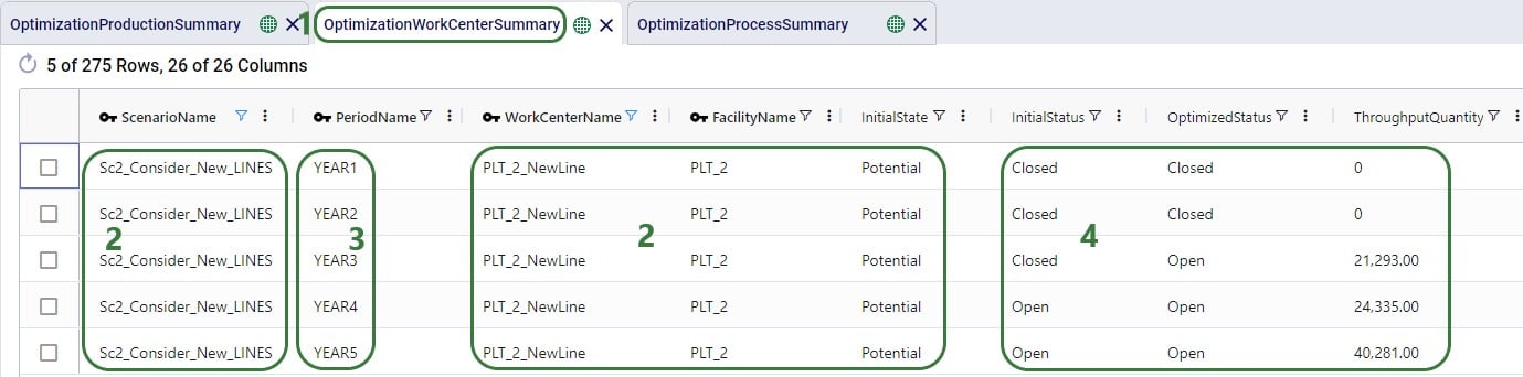
The following screenshot shows a few more output fields on the Optimization Work Center Summary output tables that have non-0 values in this model:
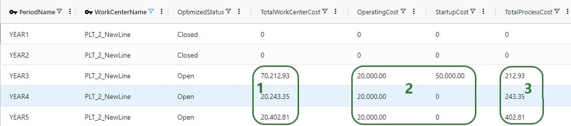
Other fields on this output table which are not shown in the screenshots are:
For all constraints in the model, the Optimization Constraint Summary can be a very handy table to check if any constraints are close to their maximum (or minimum, etc.) value to understand where the current and future bottlenecks are and likely will be. The screenshot below shows the outputs on this table for a production constraint that is applied at each of the 3 suppliers, where neither can produce more than 1 million units of RAW_MILK in any 1 year. In the screenshot we specifically look at the Supplier named SUP_3:
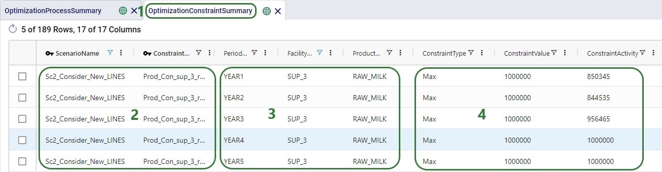
Other fields on this output table which are not shown in the screenshots are:
There are a few other output tables of which the main outputs are not related to production, but still contain several fields that result from productions. These are:
In this help article we have covered how to set up alternative Work Centers at existing locations and use the Work Center Status and Initial State fields to evaluate if including these, and from what period onwards if so, will be optimal. We have also covered how Work Center Count Constraints can be used to pick a certain amount of Work Centers to be opened/used from a set of multiple candidates, either at 1 location or multiple. Here we also want to mention that Facility Count Constraints can be used when making decisions at the plant level. Say that based on market growth in a certain region, a manufacturer decides a new plant needs to be built. There are 3 candidate locations for the plant from which the optimal needs to be picked. This can be set up as follows in Cosmic Frog:
A couple of alternative approaches to this are:
As mentioned above in the section on the Bill Of Materials input table, it is possible to set up a model where there is demand for a product that is the By-product resulting from a BOM. This does require some additional set up, and the below walks through this, while also showcasing how the model can be used to determine how much of any flexible demand for this by-product to fulfill. The screenshots show the set-up of a very simple example model built for this specific purpose.
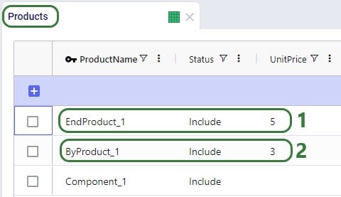
On the Products table, besides the component (for which there also is demand in this model) that goes into any BOM, we also specify:

The demand for the 3 products is set up on the Customer Demand table and we notice that 1) there is demand for the Component, the End Product, and the By-Product, and 2) the Demand Status for ByProduct_1 is set to Consider, which means it does not need to be fulfilled, it will be (partially) fulfilled if it is optimal to do so. (For Component_1 and EndProduct_1 the Demand Status field is left blank, which means the default value of Include will be used.)
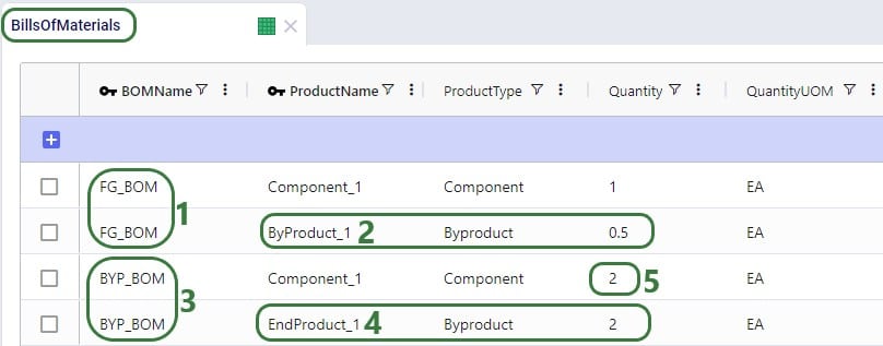
The EndProduct_1 is made through a BOM which consumes Component_1 and also make ByProduct_1 as a Byproduct. For this we need to set up a BOM:

Next, on the Production Policies table, we see that Component_1 can be created without a BOM, and:
In reality, these 2 production policies result in the same consumption of Component_1 and same production amounts of EndProduct_1 and ByProduct_1. Both need to be present however in order to be able to also have demand for ByProduct_1 in the model.
Other model elements that need to be set up are:
Three scenarios were run for this simple example model with the only difference between them the Unit Price for ByProduct_1: Baseline (price of ByProduct_1 = 3), PriceByproduct1 (Unit Price of ByProduct_1 = 1), PriceByproduct2 (Unit Price of ByProduct_1 = 2). Let’s review some of the outputs to understand how this Unit Price affects the fulfillment of the flexible demand for ByProduct_1:

The high-level costs, revenues, profit and served/unserved demand outputs by scenario can be found on the Optimization Network Summary output table:
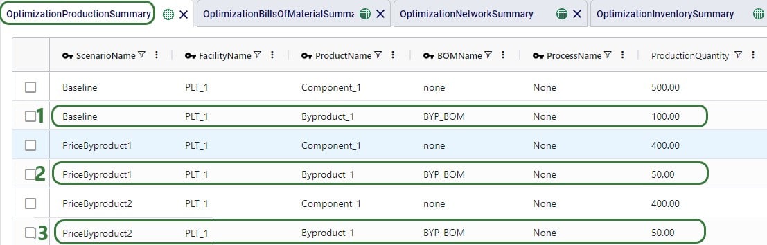
On the Optimization Production Summary output table, we see that all 3 scenarios used BYP_BOM for the production of EndProduct_1 and ByProduct_1, it could have also picked the other BOM (FG_BOM) and the overall results would have been the same.
As the Optimization Production Summary only shows the production of the end products, we will also have a look at the Optimization Bills Of Material Summary output table:
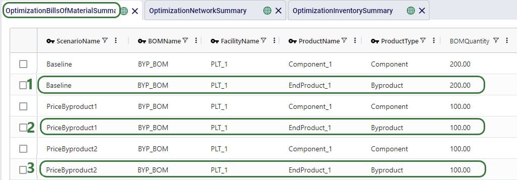
Lastly, we will have a look at the Optimization Inventory Summary output table:

Note that had the demand for Byproduct_1 been set to Include rather than Consider in this example model, all 3 scenarios would have produced 100 units of it to fulfill the demand, and as a result have produced 200 units of EndProduct_1. 100 of those would have been used to fulfill the demand for EndProduct_1 and the other 100 would have stayed in inventory, like we saw in the Baseline scenario above.
In a supply chain model, sourcing policies describe how network components create and order necessary materials. In Cosmic Frog, sourcing rules & policies appear in two different table categories:
In this section, we will discuss how to use these Sourcing policy tables to incorporate real-world behavior. In the sourcing policy tables we define 4 different types of sourcing relationships:
First we will discuss the options user has for the simulation policy logic used in these 4 tables and the last section covers the other simulation specific fields that can be found on these sourcing policies tables.
Customer fulfillment policies describe which supply chain elements fulfill customer demand. For a Throg (Simulation) run, there are 3 different policy types that we can select in the “Simulation Policy” column:
If “By Preference” is selected, we can provide a ranking describing which sites we want to serve customers for different products. We can describe our preference using the “Simulation Policy Value” column.
In the following example we are describing how to serve customer CZ_CA’s demand. For Product_1, we prefer that demand is fulfilled by DC_AZ. If that is not possible, then we prefer DC_IL to fulfill demand. We can provide rankings for each customer and product combination.
Under this policy, the model will source material from the highest ranked site that can completely fill an order. If no sites can completely fill an order, and if partial fulfillment is allowed, the model will partially fill orders from multiple sources in order of their preference.
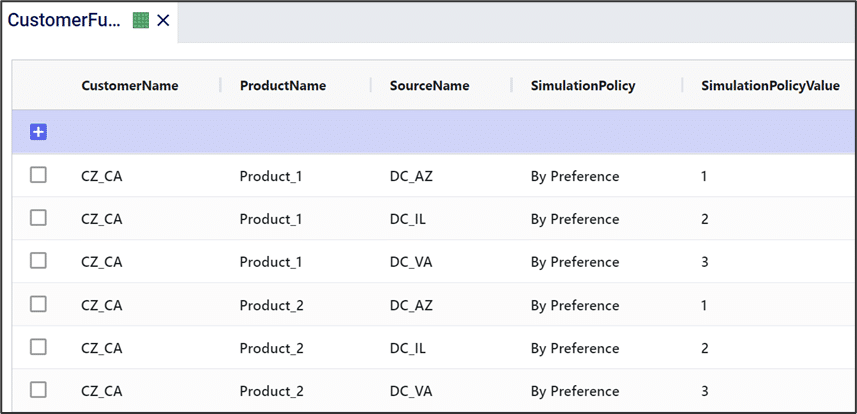
If “Single Source” is selected, the customer must receive the given product from 1 specific source, 1 of the 3 DCs in this example.
The “Allocation” policy is similar to the “By Preference” policy, in that it sources from sites in order of a preference ranking. The “Allocation” policy, however, does not look to see whether any sites can completely fill an order before doing partial fulfillment. Instead, it will source as much as possible from source 1, followed by source 2, etc. Note that the “Allocation” and “By Preference” policies will only be distinct if partial fulfillment is allowed for the customer/product combination.
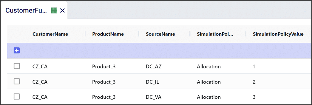
Consider the following example, customer CZ_MA can source the 3 products it puts orders in for from 3 DCs using the By Preference simulation policy. For each product the order of preference is set the same: DC_VA is the top choice, then DC_IL, and DC_AZ is the third (last) choice. Also note that in the Customers table, CZ_MA has been configured so that it is allowed to partially fill orders and line items for this customer.
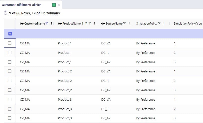
The first order of the simulation is one that CZ_MA places (screenshot from the Customer Orders table), it orders 20 units of Product_1, 600 units of Product_2, and 160 units of Product_3:
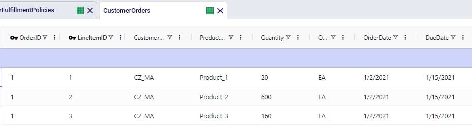
The inventory at the DCs for the products at the time this orders comes in is the same as the initial inventory as this customer order is the first event of the simulation:

When the simulation policy is set to By Preference, we will look to fill the entire order from the highest priority source possible. The first choice is DC_VA, so we check its inventory: it has enough inventory to fill the 20 units of Product_1 (375 units in stock) and the 160 units of Product_3 (500 units in stock), but not enough to fill the 600 units of product_2 (150 units in stock). Since the By Preference policy prefers to single source, it looks at the next priority source, DC_IL. DC_IL does have enough inventory to fulfill the whole order as it has 750 units of Product_1, 1000 units of Product_2, and 300 units of Product_3 in stock.
Now, if we change all the By Preference simulation policies to Allocation via a scenario and run this scenario, the outcomes are different. In this case, as many units as possible are sourced from the first choice DC, DC_VA in this case. This means sourcing 20 units of Product_1, 150 units of Product_2 (all that are in stock), and 160 units of Product_3 from DC_VA. Then next, we look at the second choice source, DC_IL, to see if we can fill the rest of the order that DC_VA cannot fill: the 450 units left of Product_1, which DC_IL does have enough inventory to fill. These differences in sourcing decisions for these 2 scenarios can for example be seen in the Simulation Shipment Report output table:

Replenishment policies describe how internal (i.e. non-customer) supply chain elements source material from other internal sources. For example, they might describe how a distribution center gets material from a manufacturing site. They are analogous to customer fulfillment policies, except instead of requiring a customer name, they require a facility name.
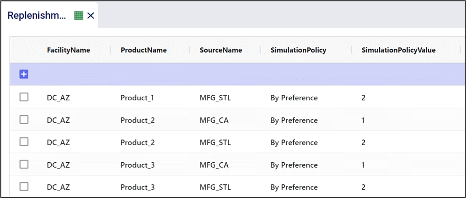
Procurement policies describe how internal (i.e. non-customer) supply chain elements source material from external suppliers. They are analogous to replenishment policies, except instead of using internal sources (e.g. manufacturing sites), they use external suppliers in the Source Name field.

Production policies allow us to describe how material is generated within our supply chain.
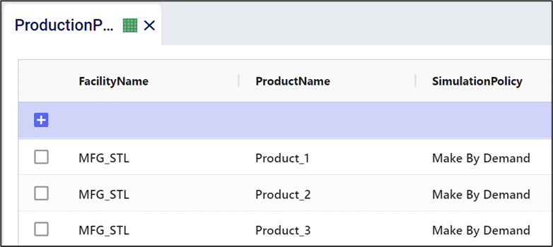
There are 4 simulation policies regarding production:
Besides setting the Simulation Policy on each of these Sourcing Policies tables, each has several other fields that the Throg Simulation engine uses as well, if populated. All 4 Sourcing Policies tables contain a Unit Cost and a Lot Size field, plus their UOM fields. The following screenshot shows these fields on the Replenishment Policies table:

The Customer Fulfillment Policies and Replenishment Policies tables both also have an Only Source From Surplus field which can be set to False (default behavior when not set) or True. When set to True, only sources which have available surplus inventory are considered as the source for the customer/facility – product combination. What is considered surplus inventory can be configured using the Surplus fields on the Inventory Policies input table.
Finally, the Production Policies table also has following additional fields: